Description of the problem

Anomaly detection is a process of detecting outliers in the data. The applications of anomaly detection includes detecting credit card fraud and spam emails. The data you will be analyzing consists of 'normal' applications and 'risky' applications for a credit card. You will use two models, called One-Class Support and Robust Covariance Estimation, to distinguish between those two classes. Unlike supervised training, the scores generated by the models only indicate a measure of distance from the 'normal' category of data. The scores can be used as the threshold for detection, not for probabilities.

The training data consists of 1,000 credit card applications with 20 feature columns and 1 label column. (Data source: UCI data repository)

What you will build

• One-Class SVM anomaly detector
• Robust Covariance Estimation

What you will learn

• Explore the dataset by using pandas, numpy, matplotlib.
• Split dataset into train, test and validation sets by using stratified sampling.
• One-Class Support Vector Machine based anomaly detector.
• Robust Covariance Estimation for detecting outliers in a Gaussian distributed dataset.

• pandas
• numpy
• matplotlib
• sklearn

Since the original dataset does not have column names, remember to initialize the column names before next step. The dataset contains 8 numeric variables and 13 categorical variables.

Now check again the variables, are they all meaningful for the model? You can drop the variable that you think will not help you build the detector.

In the following steps, we will be using One-Class SVM predict function in sklearn to generate the output. It will return +1 or -1 to indicate whether the data is an "inlier" or "outlier" respectively. To make the label value unified, it is better to replace label [1, 2] with [1, -1]. This also transforms our data from multi-class (multiple different labels) to one-class (boolean label), which is necessary when using One-Class SVM.

After cleaning the data, the top 5 rows in the dataset (part of the columns) should be like this:

In this step, we need to split the data several times for different use.

1. Split the data into "normal" transactions label_normal (label=1) and "risky" transaction label_risky (label=-1) for future evaluation.
2. Split the data into training (80%) and test (20%) using stratified sampling for modeling.
3. Split the features and labels into X_train, X_test, y_train and y_test.
4. Select rows containing "normal" transactions X_train_normal from train set to train the detector.
5. Split the train set into training (80%) and validation (20%) sets using stratified sampling for hyperparameter tuning
6. Select rows containing "normal" transactions X_training_normal from training set.

One-Class Support Vector Machine (SVM) is a binary classifier where the training data has examples of only one class (normal data). The model separates the collection of training data from the origin by using maximum margin.

First, you need to tune the hyperparameters. You can specify a grid of value for each of the parameters. Then, use the training data which consists of examples from a single class to fit an untrained model, and optimize the scores (F-score, recall, precision, AUC), using validation data which consists of examples from both classes. Finally, you will find the best settings for the model.

For One-Class SVM, parameters ‘tol' (Tolerance for stopping criterion) and ‘nu' (an upper bound on the fraction of training errors and a lower bound of the fraction of support vectors) can be used to tune the model.

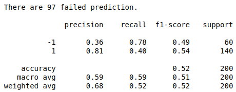
Since our goal is to detect anomaly data where label=-1, it is important to optimize F-score and and the recall. Let's select the parameter set {nu:0.01, tol:0.01}, with highest recall score of label= -1 and good F1 score(say at least 0.4). The performance result shows below:

Another way to perform outlier detection is to assume that the regular data come from a known distribution; For example, data are Gaussian distributed. From this assumption, we can try to define the "shape" of the data to define outlying observation as observations which stand far enough from the fit shape. [2]

The sklearn provides an object covariance.EllipticEnvelope that fits a robust covariance estimate to the data, and thus fits an ellipse to the central data points, ignoring points outside the central mode.

Before building the model, the first thing you need to do is hyperparameter tuning. For EllipticEnvelope, you can try to find the best value of ‘contamination' ( The amount of contamination of the data set) to tune the model.

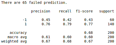
As we explained in the previous step, you need to find a model which has a high F-score and recall score. In the notebook, select parameter contamination=0.17 to build the model. The performance of the model is shown below:

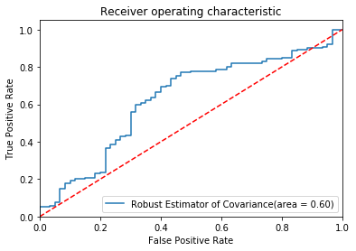
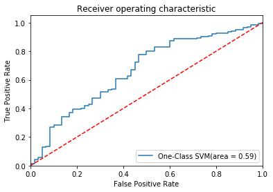
To visualize the performance, you can plot the ROC curve of two models in one plot.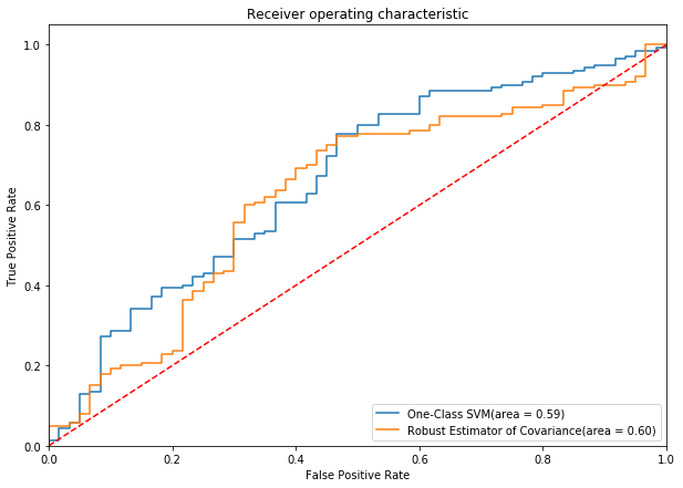

Area under the ROC curve provides a good way to measure the discriminatory power of the anomaly detectors. Based on the graph, we can learn that the One-Class SVM and Robust Estimator of Covariance have comparable performance in anomaly detection. In terms of -1 label detection, you can see from the table below that One-Class SVM does a much better job with recall score of -1 0.78.

Result table

1. Azure ML Team for Microsoft. (2014, September 2). Anomaly Detection: Credit Risk.
2. Scikit Learn. 2.7. Novelty and Outlier Detection.