Description of the problem
Synthesized data is in nature a noise-added copy of the raw data, which can capture the main pattern in the original data but preserve privacy at the same time. It is necessary to have ways to easily generate synthesized data based on customized criteria but also have methods to evaluate the similarity between the raw data and the synthesized one. In this project, you will learn three implementations, including DataSynthesizer, SDV and Synthpop to generate synthesized datasets. You will also compare the similarity with graphical and statistical approaches, and their performances by using machine learning methods. In this exercise, we will use loan data from LendingClub, a website that connects borrowers and investors over the internet. The dataset is in the file Loans.csv under folder dataset.
What you will build
- Data Generator
- Attribute Comparison
- Machine Learning Performances Comparison
What you will learn
- Generate synthesized data with DataSynthesizer, SDV and Synthpop
- Compare attributes similarity with graphical and statistical methods
- Evaluate machine learning performances between real data and synthesized data
- pandas
- numpy
- matplotlib
- ploty
- seaborn
- sklearn
- Pytorch, torch_two_sample (Optional, currently not available)

This implementation provides three different ways for data generation:
- Random Mode: Each data field would be assumed drawn from uniform distribution
- Independent Mode: Each data field maintains the distribution of the raw field
- Correlated Mode: Similar to Independent Mode, this mode allows data fields to capture correlations among each other.
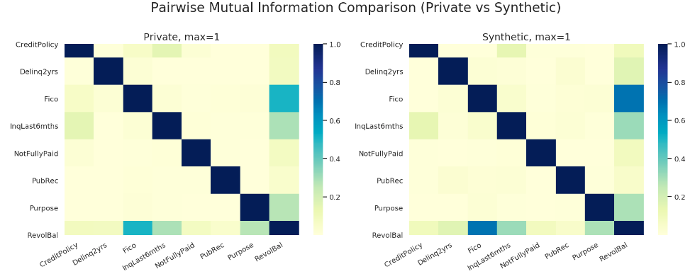
The following is a mutual information heatmap between real data and synthetic data by Correlated Mode. More comparisons can be found in section Attribute Comparison.
All generated data would be saved under the folder named "outDataSynthsizer".
SDV is a powerful synthetic data generator that can generate multiple relational tables, but in this case, we only demonstrate data generation for a single table. However, the workflow used here should be applied to multiple relational tables.
This implementation method uses Gaussian Copula at the back, and thus it is necessary to provide some external information to the tool, such as the data type. (eg. The data type can be numerical(continuous/discrete) or categorical.) This external information is called metadata, which is the data that describes other data.
SDV offers an easy-to-use method, the Metadata Module, helping users to create metadata for further processing. In addition, you may also create some useful functions to make metadata creation even more efficient. In this case, function type_infer is designed to infer the data type for each data field.
When synthetic data is generated by SDV module, you only need to provide the following two required parameters:
- Metadata: description of real data
- Tables: collection of real data
You should always be aware that the synthetic data type may be different from real data. Therefore, we should do a simple formatting over the synthetic data before saving synthetic data. With [pandas.astype] method, it is easily achieved. And output is saved at folder "outSDV".
This one is probably the easiest one to use among the three. What you have to provide is only the modeling method. Here, we use the "parametric" method, which is a method that automatically finds the best modeler for each data field. However, it is also possible to arbitrarily specify modeling methods and add more rules during modeling.
The synthesized data will be saved as dataframe named "syn" in the modeler. And the output is saved in folder "outSynthpop".
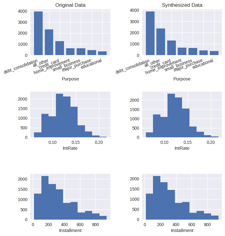
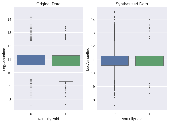
In this section, we start off with histogram for numerical data and frequency bar chart for categorical data to visualize the distributions of each data field between synthetic data and real data.
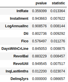
Secondly, we use statistical approaches to measure the similarity between synthetic data and real data. For numerical data, Two-sample Kolmogorov–Smirnov test is applied and KL Divergence Test is for categorical data. These two methods only work with univariate variables.
Another method named MMD test can be used for either univariate variable or multivariate variables. And thus MMD can be an overall measure for similarity between real data and synthetic data.
Keep in mind that you have to have the right directory where real data and synthetic data are located. In this way, it is easy to switch between different synthetic data and you can compare it with the real data. This idea is also applied in the Machine Learning Performances section.
Graphical Comparison :
Distribution Plot:
Here only [Purpose], [IntRate], and [Installment] are displayed, but you can easily see plots for other data fields.
Boxplot:
Statistical Testing:
Two-sample Kolmogorov–Smirnov Test (Numerical Data):
KL Divergence Test (Categorical Data, only p value returned):

MMD Test (Numerical Data,univariate and multivariate):
MMD test is a distance-based testing statistics, and thus the interpretation for it is that if testing result is to zero, then similarity is high, and vice versa.
Measure for single data field of numerical variable:
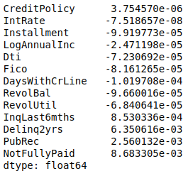
Measure for overall similarity:

Given all testing statistics/p values are close to zero, we can conclude that the real data and synthetic data is fairly close/similar to each other.
In this section, we will perform regression and classification by arbitrarily picking up the responsive variables. Categorical data fields can be used for classification while numerical data fields for regression.
In order to perform different machine learning methods with different responsive variables and compare their performances, a few functions are defined in the modelling.py file. They are some high-level wrap up of sklearn classes.
Firstly, we use "NotFullyPaid" and "IntRate" for classification and regression respectively.

Before implementing any machine learning steps, it is necessary to preprocess the data by dealing with filling missing values or detent outliers. Given the Loan.csv data used here, dummy variable creation and scaling is applied. Different preprocessing techniques may be required depending on the data you are using.
Thirdly, choose regressors and classifiers to compute the evaluation metrics. Again, refer to the modelling.py file for more details.
Classification Performance (Real Data VS Synthesized by Synthpop) :
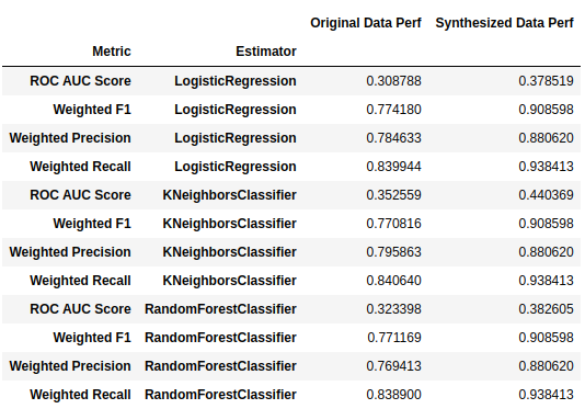
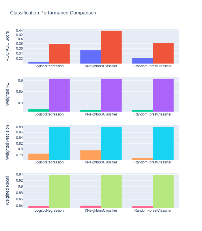
Classification performance over synthetic data is better, and the reason for that is the underlying method synthpop has been applied. Synthpop's generating method can be summarized in the following procedure:
A column of x_i is selected and the distribution of this variable, conditional on some given information is estimated. Then the next column x_i+1 is selected and its distribution is estimated conditional on given information and the column of x_i already selected. The distribution of subsequent columns are estimated conditional on given information and all previous columns.
In short, the responsive variable would be generated based on other columns. This means it is classifiable by those other columns. It is not surprising to see performance improvement over synthetic data.
Regression Performance (Real Data VS Synthesized by Synthpop) :
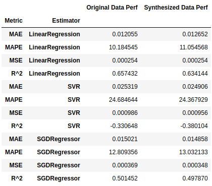
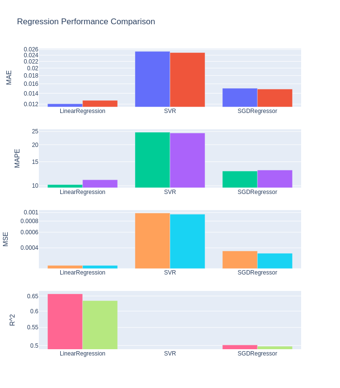
Based on conclusion from classification performance comparison above, it is expected that performance over synthetic data is not worse than real data. However, performance for regression problems is fairly comparable. There is no big improvement or negative impact. Still the responsive variable is generated by some columns, but unlike categorical variable, numerical variable would be more volatile. Therefore a big improvement would be hard to get.