Description of the problem
Lending Club strives to connect borrowers with investors through our online marketplace.
The goal is to predict the interest rates that Lending Club should use, based on previous borrowers data they have. Whether or not a client will repay a loan or have difficulty is a critical business need. In this project, we are going to see some models that the machine learning community can develop to help organizations like Lending Club.
What you will build
- Visualizations to understand the Lending Club Dataset
What you will learn
- Module 1: Perform Exploratory Data Analysis (EDA) on the dataset
The experimentation will be done in Jupyter Notebooks, primarily in Python3.6.
- pandas
- numpy
- matplotlib
- seaborn
- sklearn
In this project, we are going to use the Lending Club loan dataset. The provided file is a cleaned version of the original Lending Club dataset available at Kaggle. The files provided includes a file containing the description of the features, LCDataDictionary, and the data file named LendingClubLoan.csv.
The original version of the dataset is about 230mb. The version provided is a subset of 9999 samples of the cleaned dataset. Let us first take a look at some of the features in the given dataset. The entire list can be found in the jupyter notebook.
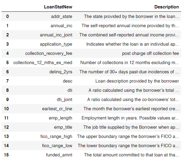
Here is a look at some of the entries in the dataset:

Exploratory Data Analysis (EDA) is an open-ended process where we calculate statistics and make figures to find trends, anomalies, patterns, or relationships within the data. The goal of EDA is to learn what our data can tell us. It generally starts out with a high level overview, then narrows into specific areas as we find intriguing areas of the data. The findings may be interesting in their own right, or they can be used to inform our modeling choices, such as by helping us decide which features to use.
Types of feature
This particular dataset has equal number of numeric and categorical features, 4 each.
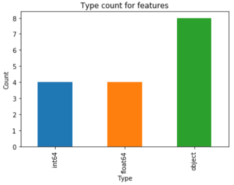
Numerical features
The numerical features include 'loan_amnt', 'int_rate', 'installment', 'annual_inc', 'dti', 'delinq_2yrs',
'inq_last_6mths', 'loan_status_Binary'.
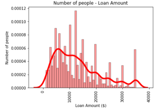
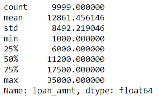
Summary of Loan amounts
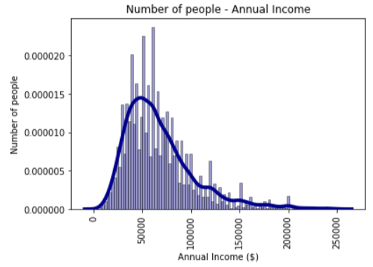
Summary of annual incomes

Categorical features
The cleaned dataset has 8 categorical features that can affect the predictions.
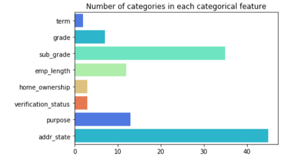
Categorical data is best processed by algorithms when converted to numerical format.The most common way is by mapping each category to an integers. Ex. [A, B, C] can be mapped to [0, 1, 2]. Another way is one-hot encoding which we will look into while building the models.
For example, the following is the conversion for ‘purpose' feature:
0: 'car'
1: 'credit_card'
2: 'debt_consolidation'
3: 'home_improvement'
4: 'house'
5: 'major_purchase'
6: 'medical'
7: 'moving
8: 'other'
9: 'renewable_energy'
10: 'small_business'
11: 'vacation'
12: 'wedding'
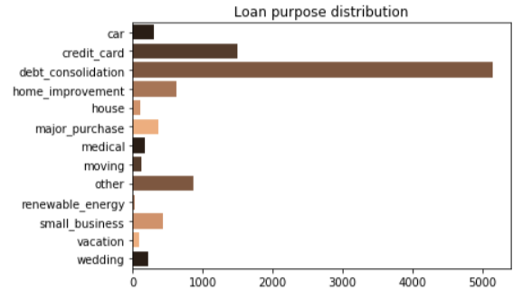
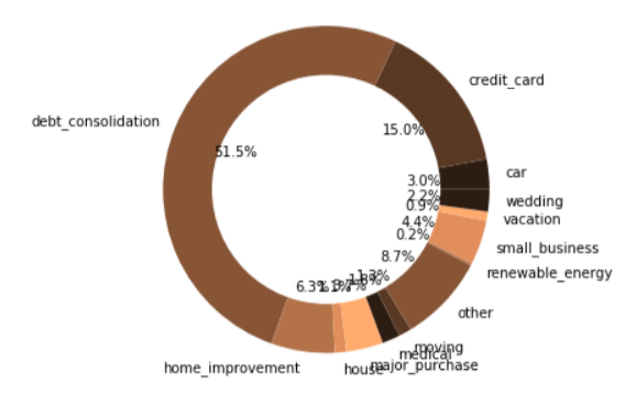
Summary of loan purposes
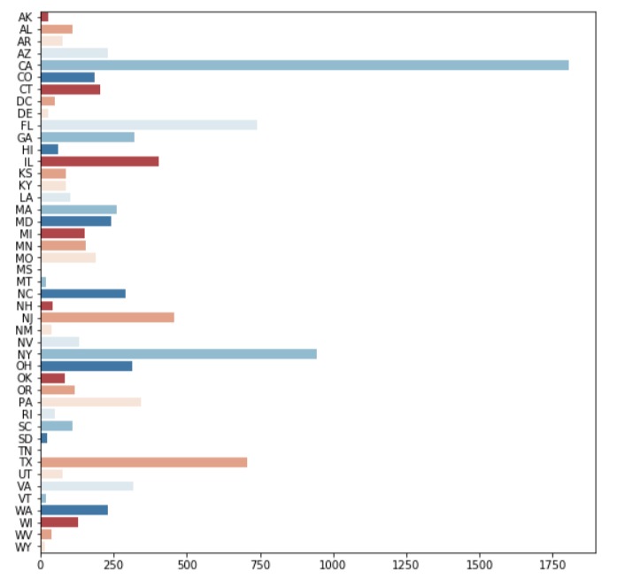
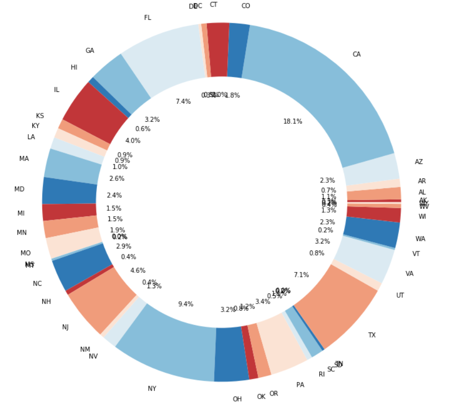
Summary of state
California, Florida, New York and Texas have the highest number of borrowers.
We can calculate the correlation matrix for the given numerical features to see the relation or dependency of features among themselves. Each cell in the matrix describes the Pearson Correlation coefficient, a value between -1 and 1. A correlation coefficient indicates the extent to which dots in a scatterplot lie on a straight line. This implies that we can usually estimate correlations pretty accurately from nothing more than scatterplots. +1 is highly linearly related and -1 is highly negatively linearly related. A fractional number indicates deviation from a linear trend.
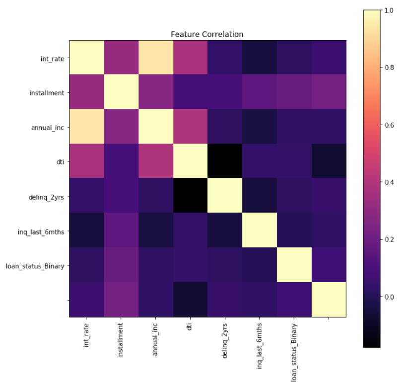
For the given dataset, it is evident from the correlation matrix that the installment is somewhat related to all other numerical features. Also, interest rate, annual income and dti have some sort of linear relationship.
Multicollinearity occurs when your model includes multiple factors that are correlated not just to your response variable, but also to each other. It may increases the standard errors of the coefficients which will make some variables statistically insignificant when they should be significant. In order to select actual significant features, you may need to remove highly correlated predictors from the model.
After dropping highly correlated features, remember to convert the categorical variables into dummy variables.
In this particular dataset, even though interest rates and annual income are correlated, we will keep both as they are very domain specific and important to the use case.
A complete overview of the dataset can be found at this link.