Convex optimization is a subfield of mathematical optimization that studies the problem of minimizing convex functions over convex sets. Whereas many classes of convex optimization problems admit polynomial-time algorithms, mathematical optimization is in general NP-hard. Convex optimization has applications in a wide range of disciplines, such as automatic control systems, estimation and signal processing, communications and networks, electronic circuit design,data analysis and modeling, finance, statistics (optimal experimental design), and structural optimization. With recent advancements in computing and optimization algorithms, convex programming is nearly as straightforward as linear programming.

What you will build

In this data lab, you will encounter optimization problems under various circumstances including:

1. Portfolio optimization
2. Worst-case risk analysis
3. Scheduling problems
4. Other optimization problems

What you will learn

Your learning objectives are:

1. You will learn how to set up constraints and mathematical models for portfolio optimization using ‘cvxpy' and Google OR-Tools.
2. You will learn to use Python to write concrete numerical scripts for the whole portfolio optimization process.

What you will need

You will need to:

1. If you are doing the experiment on your own machine, you should first install Python 3.5, Jupyter notebook and the necessary packages list in the first cell of the notebook on your local machine. QuSandbox has all the packages and installs in the experiment
2. You need to understand the basic concepts for optimization problems. Don't worry if you are new in this area. Check the resource link below in ‘Prerequisite Knowledge' part.

What packages you need to install

Make sure you have installed Python 3.5, Jupyter notebook and the following packages. If you need any guide, check the links below:

1. Python installation: https://www.python.org/downloads/release/python-366/
2. Jupyter notebook installation: http://jupyter.readthedocs.io/en/latest/install.html
3. Package installation example: https://pandas.pydata.org/pandas-docs/stable/install.html
4. Cvxpy installation ducumentation: https://www.cvxpy.org/install/index.html
5. Necessary packages: Pandas, numpy, cvxpy, matplotlib

Where you can find the solution

You can find sample code this exercise is in the QuSandbox data lab named ‘CVX Short Course'. The directory for the sample notebooks is ‘work/cvx_short_course/applications'.

Optimization Problem

In mathematics and computer science, an optimization problem is the problem of finding the best solution from all feasible solutions. Optimization problems can be divided into two categories depending on whether the variables are continuous or discrete. An optimization problem with discrete variables is known as a discrete optimization. In a discrete optimization problem, we are looking for an object such as an integer, permutation or graph from a finite (or possibly countably infinite) set. Problems with continuous variables include constrained problems and multimodal problems.

If you want to find more information about optimization problems, you find systematic introduction here: https://en.wikipedia.org/wiki/Optimization_problem

Portfolio optimization

Portfolio optimization is the process of selecting the best portfolio (asset distribution), out of the set of all portfolios being considered, according to some objective. The objective typically maximizes factors such as expected return, and minimizes costs like financial risk. Factors being considered may range from tangible (such as assets, liabilities, earnings or other fundamentals) to intangible (such as selective divestment).

Check here for more information: https://en.wikipedia.org/wiki/Portfolio_optimization

Portfolio Optimization example

In the portfolio_optimziation.ipynb, one will see how to do portfolio optimization using CVXPY. Here is a brief introduction of the problem:

• One would allocate his/her money to different assets for investment.
• A vector called ‘portfolio allocation vector' will be used to decide the percentage of the total capital in each asset.
• One will build mathematical constraints for this optimization problem to minimize the risk.
• In this example, we are dealing with a classical (Markowitz) portfolio optimization problem and its variations.

Optimization results:

One can see the expected return versus standard deviation plots for the optimization solutions.

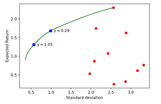
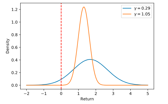
Next, we can see the expected return distributions for the two risk aversion values marked on the trade-off curve. Notice that the probability of a loss (the area under the curve to the left of the red dotted line) is near 0 for the high risk aversion value and far above 0 for the low risk aversion value.

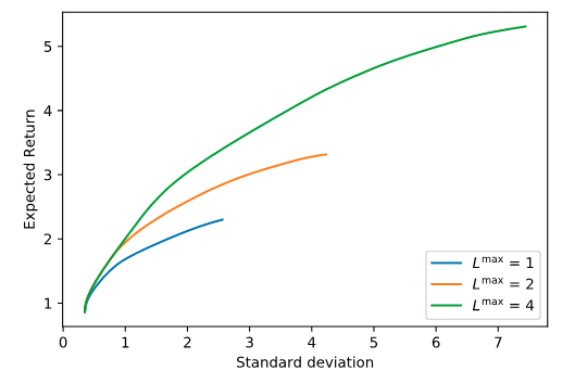
Then we compute and plot optimal risk-return trade-off curves for different leverage limits. Notice that more leverage increases returns and allows greater risk.

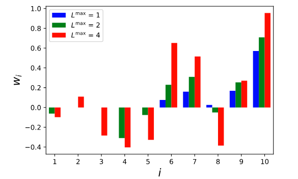
We next examine the points on each trade-off curve. We plot the amount of each asset held in each portfolio as bar graphs. (Negative holdings indicate a short position.) Notice that some assets are held in a long position for the low leverage portfolio but in a short position in the higher leverage portfolios.

Worst case risk analysis example

In this example we do worst-case risk analysis using CVXPY. Our setting is a single period Markowitz portfolio allocation problem. Below is the brief background information.

• We have a fixed portfolio allocation.
• The return covariance is not known, but we believe it is in a convex set of possible covariance matrices.
• The risk is a linear function of return covariance.
• We can compute the worst (maximum) risk, over all possible covariance matrices by solving the convex optimization problem

If the worst-case risk is not too bad, you can worry less. If not, you'll confront your worst nightmare.

First one need to create date for this experiment:

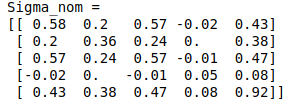
Next, we form and solve portfolio optimization problem. Here we minimize risk while requiring a 0.1 return. We can get the portfolio weights as follows:

In the end, we can form and solve worst-case risk analysis problem.

Job shop problem example

One common scheduling problem is the job shop, in which multiple jobs are processed on several machines. Each job consists of a sequence of tasks, which must be performed in a given order, and each task must be processed on a specific machine. For example, the job could be the manufacture of a single consumer item, such as an automobile. The problem is to schedule the tasks on the machines so as to minimize the length of the schedule—the time it takes for all the jobs to be completed.

There are several constraints for the job shop problem:

• No task for a job can be started until the previous task for that job is completed.
• A machine can only work on one task at a time.
• A task, once started, must run to completion

A solution to the job shop problem is an assignment of a start time for each task, which meets the constraints given above. The diagram below shows one possible solution for the problem:

The Google OR-Tool gives the optimal scheduling solutions as follows:

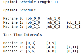
The length of the optimal schedule is 11, which is an improvement over the solution shown previously. The optimal schedule is displayed for each machine, where Job_i_j represents the jth task for job i.

Here's the timeline for the optimal schedule.

Nurse scheduling problem example

A nurse scheduling problem In the next example, a hospital supervisor needs to create a schedule for four nurses over a three-day period, subject to the following conditions:

• Each day is divided into three 8-hour shifts.
• Every day, each shift is assigned to a single nurse, and no nurse works more than one shift.
• Each nurse is assigned to at least two shifts during the three-day period.

Then you need to assign nurses to shifts Next, we show how to assign nurses to shifts subject to the following constraints:

• Each shift is assigned to a single nurse per day.
• Each nurse works at most one shift per day.

In the end, one will see the one of the scheduling problems solutions as follows:

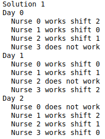
One can view more solutions in the sample notebook. One will also see how we can confirm the correctness of optimization solution in the notebook.