Portfolio optimization is the process of selecting the best portfolio (asset distribution), out of the set of all portfolios being considered, according to some objective. The objective typically maximizes factors such as expected return, and minimizes costs like financial risk. Factors being considered may range from tangible (such as assets, liabilities, earnings or other fundamentals) to intangible (such as selective divestment). This exercise is a tutorial to show you how to leverage Python to solve portfolio optimization problem and compare the risk and return of the target asset distribution.
What you will build
You will build various examples using the package ‘cvxportfolio' to understand the optimization and simulation process, including:
- collecting historical assets transaction data using Quandl;
- defining portfolio positions, weights, trades, post-trade portfolio, and portfolio returns;
- building transaction and holding cost model;
- various simulation methods.
What you will learn
Your learning objectives are:
- You will learn the standard process to solve and simulate a portfolio optimization problem.
- You will learn how to set up constraints and mathematical models for portfolio optimization using ‘cvxportfolio'.
- You will learn to use Python to write concrete statistical scripts for the whole portfolio optimization process.
What you will need
You will need to:
- If you are doing the experiment on your own machine, you should first install Python 3.5, Jupyter notebook and the necessary packages list in the first cell of the notebook on your local machine. QuSandbox has all the packages and installs in the experiment
- You need to understand the basic concepts for portfolio optimization. Don't worry if you are new in this area. Check the resource link below in ‘Prerequisite Knowledge' part.
- You will need a Quandl account with the access key to download data. To use it in our data lab, you will enter the corresponding information using our ModelRisk Platform.
What packages you need to install
Make sure you have installed Python 3.5, Jupyter notebook and the following packages. If you need any guide, check the links below:
- Python installation: https://www.python.org/downloads/release/python-366/
- Jupyter notebook installation: http://jupyter.readthedocs.io/en/latest/install.html
- Package installation example: https://pandas.pydata.org/pandas-docs/stable/install.html
- Cvxportfolio installation ducumentation: http://cvxportfolio.org/install/index.html
- Necessary packages: Pandas, numpy, quandl, cvxpy, cvxportfolio, matplotlib
Where you can find the solution
You can find sample code this exercise is in the QuSandbox data lab named ‘Cvxportfolio-Course'. The directory for the sample notebooks is ‘work/cvxportfolio/examples'.
Portfolio optimization
Portfolio optimization is the process of selecting the best portfolio (asset distribution), out of the set of all portfolios being considered, according to some objective. The objective typically maximizes factors such as expected return, and minimizes costs like financial risk. Factors being considered may range from tangible (such as assets, liabilities, earnings or other fundamentals) to intangible (such as selective divestment).
Check here for more information: https://en.wikipedia.org/wiki/Portfolio_optimization
Convex optimization Problem
Convex optimization is a subfield of mathematical optimization that studies the problem of minimizing convex functions over convex sets. Whereas many classes of convex optimization problems admit polynomial-time algorithms, mathematical optimization is in general NP-hard. The mathematical model of portfolio optimization here is a convex optimization problem provided risk, trade, and hold functions/constraints.
If you want to find more information about convex optimization problems, you find systematic introduction here: https://web.stanford.edu/class/ee364a/lectures/problems.pdf
In addition, you can find the exact mathematical models and more information in the reference paper:
https://web.stanford.edu/~boyd/papers/cvx_portfolio.html
Backtest
Backtesting is a term used in modeling to refer to testing a predictive model on historical data. Backtesting is a type of retrodiction, and a special type of cross-validation applied to previous time period(s).
Check here for more information: https://en.wikipedia.org/wiki/Backtesting
HelloWorld.ipynb shows a basic usage of the simulation and (single period) optimization objects.
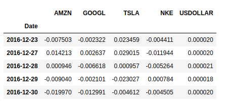
Download historical data from Quandl
In this example, you will first download the assets data from Quandl using your own access key.
Preprocess data
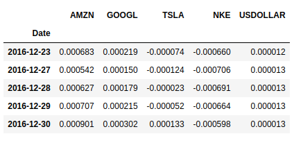
Then you will compute rolling estimates of the first and second moments of the returns using a window of 250 days. We shift them by one unit (so at every day we present the optimizer with only past data).
Define cost models and the single period optimization policy
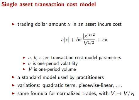
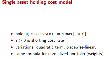
Here we define the transaction cost and holding cost model (sections 2.3 and 2.4 the reference paper). The data can be expressed as
- a scalar (like we're doing here), the same value for all assets and all time periods;
- a Pandas Series indexed by the asset names, for asset-specific values;
- a Pandas DataFrame indexed by timestamps with asset names as columns, for values that vary by asset and in time.
We define the single period optimization policy (section 4 of the reference paper). Trading policy is shaped by selection of objective terms, constraints, hyper-parameters.
Backtest
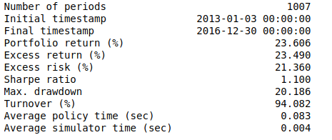
We run a backtest, which returns a result object. By calling its summary method we get some basic statistics. Below is the summary of the backtest results.
Visualize simulation results
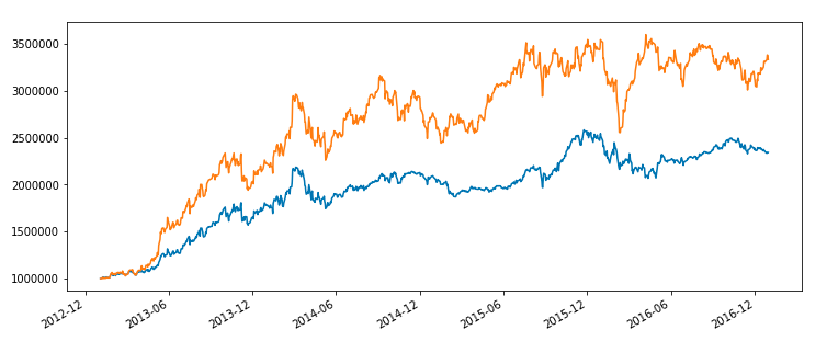
Below is the total value of two different portfolios in time.
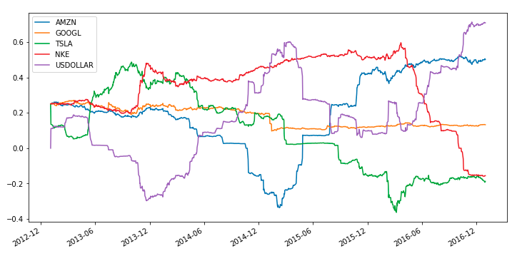
We can also plot the weights vector of the portfolio in time.
SinglePeriodOptimization.ipynb iprovides a more advanced example of the single period optimization framework, with search of optimal hyper-parameters.
Build optimization model and simulator
In this example, we first do the same steps as we did in the basic example:
- Load data and preprocess data
- Build cost model and optimization policies
Next, we start to tune the hyperparameters for the optimization model in three different search sections.
SPO coarse search
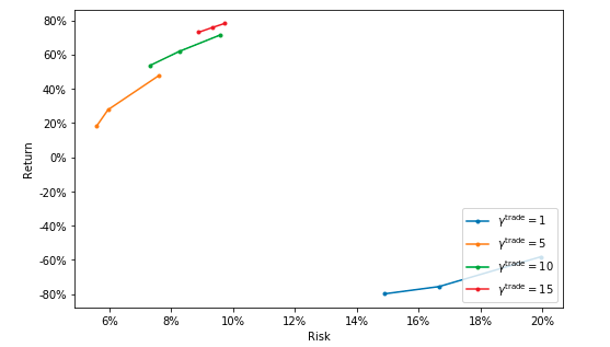
In this section, we set a coarse search with hyperparameters with significant differences to find a relatively reasonable interval for the next search section. Below you can see a return-risk trade-off plot with different trade cost hyperparameters.
SPO fine Search
In this section, we will perform a more accurate search for the trade cost parameter.
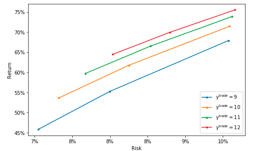
SPO Pareto search
In the last section, we do a grid search to get a Pareto optimal frontier of the portfolio optimization problem.
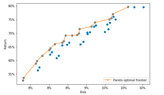
This tutorial present a few example applications built with CVXPortfolio. One can also see detail information in the reference paper.
- HelloWorld: basic usage of the simulation and (single period) optimization objects.
- DataEstimatesRiskModel: download and clean the data used for the examples in our paper. (Its output files are available in the data folder of the repo.)
- PortfolioSimulation: simple simulation of a portfolio rebalanced periodically to a target benchmark.
- SinglePeriodOptimization: example of the single period optimization framework, with search of optimal hyper-parameters.
- SolutionTime: analysis of execution time of the simulation and optimization code.