Last Updated: 07/10/2020
The code can be accessed here.
What is Explainability of Machine Learning models?
‘Black box' is often synonymous with recent machine learning models. These cannot be understood by people. Models, such as deep neural networks and large ensembles, are achieving impressive accuracy on various tasks. However, as machine learning is increasingly used to inform high stakes decisions, explainability and interpretability of the models is becoming essential. There are many ways to explain: data vs. model, directly interpretable vs. post hoc explanation, local vs. global, static vs. interactive; the appropriate choice depends on the persona of the consumer of the explanation.
Explainable AI/ML refers to methods and techniques in the application of artificial intelligence technology such that the results of the solution can be understood by humans. It contrasts with the concept of the "black box" in machine learning where even their designers cannot explain why the AI arrived at a specific decision.
Comprehensibility and Understandability are very closely related to this concept and it would be good to understand them as well. Understandability refers to the feature of a learning model where a user can understand the model's function (how the model works) without any explanations regarding the internal processes occurring in the learning model. It is similar to the term Intelligibility in the context of AI. Comprehensibility signifies the ability of a learning model to depict its learned knowledge in a way such that it is understandable to the user.
For this application, we use IBM's AIX360. Here we demonstrate 3 different perspectives for the interpretation of the model. Note: All the methods will be explained in depth in the following parts. Look at the overview for now.
- Data Scientist's view: In evaluating a machine learning model for deployment, a data scientist would ideally like to understand the behavior of the model as a whole, not just in specific instances
- Boolean Rule based system
- Logistic Regression based rules
- Loan Officer's view: Loan officer might be interested in generating explanations in the form of selecting prototypical or similar user profiles to an applicant in question. This may help her/him understand the decision of an applicant's HELOC application being accepted or rejected in the context of other similar applications.
- Prototypical Explanations
- Customer's view: Customers would like to understand why they do not qualify for a line of credit and if so what changes in their application would qualify them. On the other hand, if they qualified, they might want to know what factors led to the approval of their application.
- Contrastive Explanations
What will you learn?
- What is Explainability of Machine Learning models?
- What are some of the methods available to interpret the results/models?
- What are the different perspectives regarding understanding ML models?
The application demonstrates 2 datasets:
- HELOC dataset
- Lending Club dataset
HELOC Datset
The FICO HELOC dataset contains anonymized information about home equity line of credit (HELOC) applications made by real homeowners. A HELOC is a line of credit typically offered by a US bank as a percentage of home equity (the difference between the current market value of a home and the outstanding balance of all lines, e.g. mortgages). The customers in this dataset have requested a credit line in the range of USD 5,000 - 150,000. The machine learning task we are considering is to use the information about the applicant in their credit report to predict whether they will make timely payments over a two year period. The machine learning prediction can then be used to decide whether the homeowner qualifies for a line of credit and, if so, how much credit should be extended.
The HELOC dataset and more information about it, including instructions to download, can be found here.
'RiskPerformance' is the target variable here. The meaning of other columns can be found here

Lending Club Dataset
Looking into the dataset, the files contain complete loan data for all loans issued through the 2007-2015, including the current loan status (Current, Late, Fully Paid, etc.) and latest payment information. Additional features include credit scores, number of finance inquiries, address including zip codes, and state, and collections among others. There are 145 columns with information representing individual loan accounts. Each row is divided by an individual loan id and member id, of course, for the interest of privacy each member id has been removed from the dataset. Below you can identify some (not all) columns within the dataset.

‘Loan_status' is the target variable here. The meaning of other variables can be found here.
Let's look at the problem from completely different angels.
- Data Scientist's
- Loan Officer's
- Consumers
Data Scientist's PoV
In evaluating a machine learning model for deployment, a data scientist would ideally like to understand the behavior of the model as a whole, not just in specific instances (e.g. specific loan applicants). This is especially true in regulated industries such as banking where higher standards of explainability may be required. For example, the data scientist may have to present the model to: 1) technical and business managers for review before deployment, 2) a lending expert to compare the model to the expert's knowledge, or 3) a regulator to check for compliance. Furthermore, it is common for a model to be deployed in a different geography than the one it was trained on. A global view of the model may uncover problems with overfitting and poor generalization to other geographies before deployment.
Loan Officer's PoV
A loan officer, rather than looking at the model, would want to check for similar applicants and understand how they performed on their credit. This may help the employee understand the decision of an applicant's HELOC application being accepted or rejected in the context of other similar applications.
Consumer's PoV
Typically, homeowners would like to understand why they do not qualify for a line of credit and if so what changes in their application would qualify them. On the other hand, if they qualified, they might want to know what factors led to the approval of their application. In this context, contrastive explanations provide information to applicants about what minimal changes to their profile would have changed the decision of the AI model from reject to accept or vice-versa (pertinent negatives).
For example, increasing the number of satisfactory trades to a certain value may have led to the acceptance of the application, everything else being the same. The method presented here also highlights a minimal set of features and their values that would still maintain the original decision (pertinent positives).
Here we demonstrate 2 methods:
- Boolean Rule Generation
- Logistic Rule Generation
Boolean Rule Generation
Boolean Rule Column Generation (BRCG) is designed to produce a very simple OR-of-ANDs rule (known more formally as disjunctive normal form, DNF) or alternatively an AND-of-ORs rule (conjunctive normal form, CNF) to predict whether an applicant will repay the loan on time (Y = 1). For a binary classification problem such as we have here, a DNF rule is equivalent to a rule set, where AND clauses in the DNF correspond to individual rules in the rule set. Furthermore, it can be shown that a CNF rule for RiskPerformance = 1 is equivalent to a DNF rule for RiskPerformance = 0.
BRCG is distinguished by its use of the optimization technique of column generation to search the space of possible clauses, which is exponential in size. To learn more about column generation, please see this NeurIPS paper .
For HELOC dataset, we find that a CNF rule for Y = 1 (i.e. a DNF for Y = 0, enabled by setting CNF=True) is slightly better than a DNF rule for Y = 1. The model complexity parameters lambda0 and lambda1 penalize the number of clauses in the rule and the number of conditions in each clause. We use the default values of 10-3 for lambda0 and lambda1 (decreasing them did not increase accuracy here) and leave other parameters at their defaults as well. The model is then trained, evaluated, and printed.

The returned DNF rule for ExternalRiskEstimate = 0 is indeed very simple with only two clauses, each involving the same two features. It is interesting to see that such a rule can already achieve 0.69 accuracy. 'ExternalRiskEstimate' is a consolidated version of some risk markers (higher is better), while 'NumSatisfactoryTrades' is the number of satisfactory credit accounts. It makes sense therefore that for applicants with more than 17 satisfactory accounts, the 'ExternalRiskEstimate' threshold dividing good and bad credit risk is slightly lower (more lenient) than for applicants with fewer satisfactory accounts.
Logistic Rule Generation
Logistic Rule Regression (LogRR) is a logistic regression model. This can improve accuracy at the cost of a more complex but still interpretable model. Specifically, LogRR fits a logistic regression model using rule-based features, where column generation is again used to generate promising candidates from the space of all possible rules.
The algorithm produces models that are weighted combinations of rules (e.g., debt < $10,000, number of accounts > 10), which give insight into loan repayment predictability. The algorithm also has the option of combining rules with linear terms, which we will use here and explain below. The model output predicts the probability of repaying on time (Y=1).
Look at the coefficient learnt for the variables for the HELOC dataset.
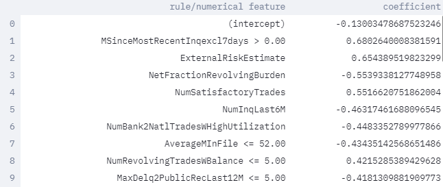

The test accuracy of LogRR is significantly better than that of BRCG and even better than the neural network in the Loan Officer and Customer sections. The LogRR model remains directly interpretable as it is a logistic regression model that uses the 36 rule-based and ordinal features shown above (in addition to an intercept term). Rules are distinguished by having one or more conditions on feature values (e.g. AverageMInFile ≤ 52.0) while ordinal features are marked by just the feature name without conditions (e.g. ExternalRiskEstimate). Being a linear model, feature importance is naturally given by the model coefficients and thus the list is sorted in order of decreasing coefficient magnitude. The list can be truncated if the user wishes to display fewer features.
Here we demonstrate the prototypical approach. The intuitive sense is that a Loan Officer, by looking at other similar applicants, might be able to decide whether to give out a credit line or not. To find the similar users, we use the ProtoDash method offered in IBM's AIX360 package.
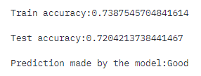
The protodash model gives out a decent accuracy. It also helps figure out the similar users and assigns a weight to the user for the HELOC dataset.
Similar applicant user profiles and the extent to which they are similar to the chosen applicant as indicated by the last row in the table below labelled as "Weight".
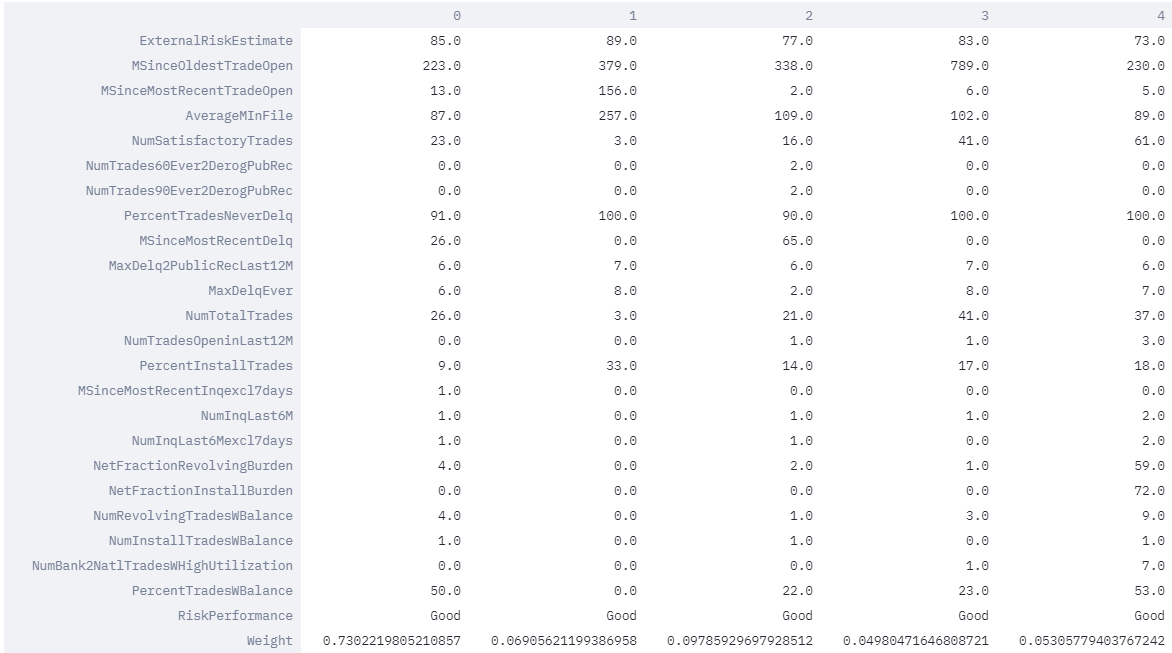
The above table depicts the five closest user profiles to the chosen applicant. Based on importance weight outputted by the method, we see that the prototype under column zero is the most representative user profile by far. This is (intuitively) confirmed from the feature similarity table above where more than 50% of the features (12 out of 23) of this prototype are identical to that of the chosen user whose prediction we want to explain. Also, the bank employee looking at the prototypical users and their features surmises that the approved applicant belongs to a group of approved users that have practically no debt (NetFractionInstallBurden). This justification gives the employee more confidence in approving the users application.
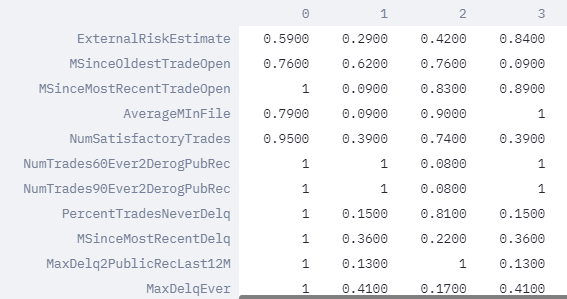
The more similar the feature of a prototypical user is to the applicant, the closer its weight is to 1. We can see below that several features for prototypes are quite similar to the chosen applicant.
Hence, the loan officer can decide.
The model for the HELOC dataset is a simple 2 layer neural network. The output is then fed into the CEMExplainer class from IBM's AIX360 package.
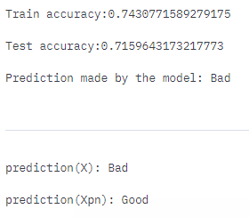
We showcase below how the decision could have been different through minimal changes to the profile conveyed by the pertinent negative. We also indicate the importance of different features to produce the change in the application status. The column delta in the table below indicates the necessary deviations for each of the features to produce this change.
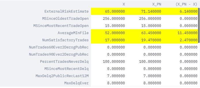
Note: This observation has been made for applicant #1272. Might differ from the observed results a bit.
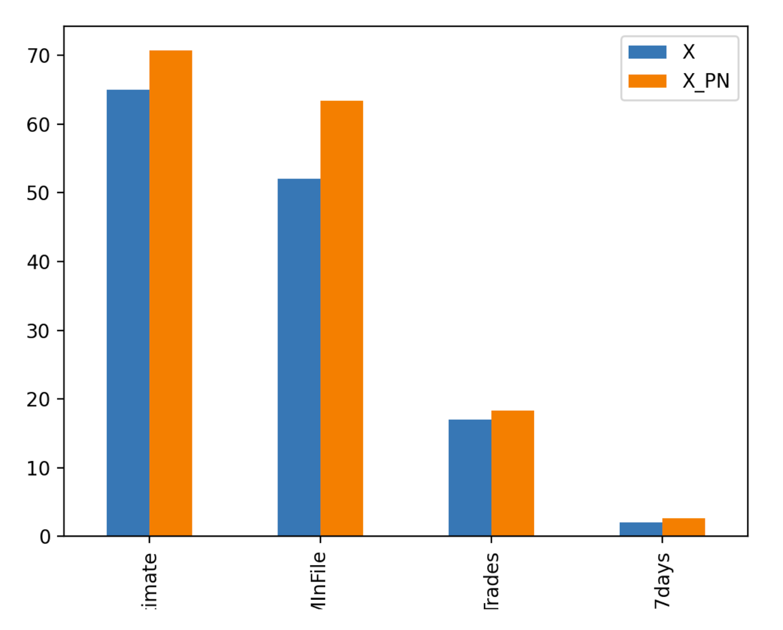
We observe that the applicant 1272's loan application would have been accepted if the consolidated risk marker score (i.e. ExternalRiskEstimate) increased from 65 to 76, the loan application was on file (i.e. AverageMlnFile) for about 65 months and if the number of satisfactory trades (i.e. NumSatisfactoryTrades) increased to little over 20.
This is how the consumers can understand why their application got rejected/accepted. And can further try to improve upon them.
- Get equipped with the HELOC dataset in the 'Data' module.
- Look into 'Data Scientist's View' to understand the model as a whole.
- Look into 'Loan Officer's View' to understand how the current applicant is related to other applicants.
- Look into 'Customer's View' to understand what excessive conditions had to be met to qualify for the line of credit.