Last Updated: 07/09/2020

The code can be accessed here.

What is Fairness in Machine Learning?

In machine learning, a given algorithm is said to be fair, or to have fairness if its results are independent of some variables we consider to be sensitive and not related with it (f.e.: gender, ethnicity, sexual orientation, etc.).

A machine learning model makes predictions of an outcome for a particular instance. (Given an instance of a loan application, predict if the applicant will repay the loan.) The model makes these predictions based on a training dataset, where many other instances (other loan applications) and actual outcomes (whether they are repaid) are provided. Thus, a machine learning algorithm will attempt to find patterns, or generalizations, in the training dataset to use when a prediction for a new instance is needed. (For example, one pattern it might discover is "if a person has a salary > USD 40K and has outstanding debt < USD 5, they will repay the loan".) In many domains this technique, called supervised machine learning, has worked very well.

However, sometimes the patterns that are found may not be desirable or may even be illegal. For example, a loan repay model may determine that age plays a significant role in the prediction of repayment because the training dataset happened to have better repayment for one age group than for another. This raises two problems: 1) the training dataset may not be representative of the true population of people of all age groups, and 2) even if it is representative, it is illegal to base any decision on a applicant's age, regardless of whether this is a good prediction based on historical data.

Research about fairness in machine learning is a relatively recent topic. Most of the articles about it have been written in the last three years. Some of the most important facts in this topic are the following:

• In 2018, IBM introduced AI Fairness 360, a Python library with several algorithms to reduce bias in a program, increasing its fairness.
• Facebook made public, in 2018, their use of a tool, Fairness Flow, to detect bias in their AI. However, said tool code is not accessible, and it is not known if it really corrects this bias.
• In 2019, Google publishes a set of tools in Github to study the effects of fairness in the long run.

For this application, we showcase following 2 packages

• IBM's AIF360: Various metrics to detect bias like Disparate Impact, Parity difference and methods to mitigate bias like Reweighig, Prejudice remover, and others are
• Aequitas Package: Various metrics like Equal Parity, Proportional Parity and other to detect bias.

What will you learn?

• What is Bias and Fairness in Machine Learning?
• What are some of the methods available for mitigating the bias?
• What are fairness metrics available and how to interpret?

This would help you navigate the documentation. The app is broadly divided into 2 parts. These parts support different packages.

The Aequitas module contains all the information for that package. The contents are as follow:

1. Dataset
2. Report
3. Fairness Metrics: Equal Parity, Proportional Parity, False Positive Rate Parity, False Discovery Rate Parity, False Negative Rate Parity, Relative Value, Absolute Value
4. Different Point of View (POVs): Data Scientist's POV, Finance Person's POV

IBM's AIF360 module contains all the information for that module. The contents are as follow:

1. Dataset
2. Methods
3. Pre-Processing Methods
4. In-processing methods
5. Post-processing methods
6. Fairness Metrics: Balanced Accuracy, Statistical Parity Difference, Equal Opportunity Difference, Average Odds Difference, Disparate Impact, Theil Index
7. Conclusion

Aequitas is an open-source bias audit toolkit for data scientists, machine learning researchers, and policymakers to audit machine learning models for discrimination and bias, and to make informed and equitable decisions around developing and deploying predictive tools.

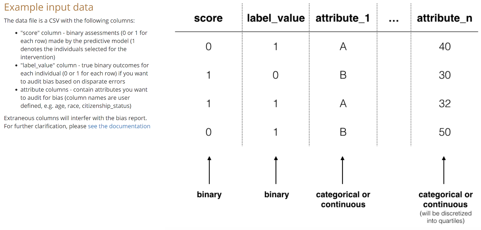
This package is model-based and checks whether the model trained is biased or not. The package requires a specific format for the report generation. The input CSV file should contain a ‘score' and ‘label_value' columns. The score is the model generated score. It can be either a class prediction or even class probability. The label_value is the ground truth values.

Dataset

The COMPAS Recidivism Risk Score Data and Analysis: Data contains variables used by the COMPAS algorithm in scoring defendants, along with their outcomes within 2 years of the decision, for over 10,000 criminal defendants in Broward County, Florida. Below you can identify some (not all) columns within the dataset.

Looking into the dataset, the files contain complete loan data for all loans issued through the 2007-2015, including the current loan status (Current, Late, Fully Paid, etc.) and latest payment information. Additional features include credit scores, number of finance inquiries, address including zip codes, and state, and collections among others. There are 145 columns with information representing individual loan accounts. Each row is divided by an individual loan id and member id, of course, for the interest of privacy each member id has been removed from the dataset. Below you can identify some (not all) columns within the dataset.

‘Loan_status' is the target variable here. The meaning of other variables can be found here.

Report

The aequitas package offers functionalities as a web-app as well as from command line to generate the report. The packages, not only creates a PDF document but also a .csv file with all the values. In the most simplest terms, the .csv//PDF can be thought of a large pivot table representing the data.

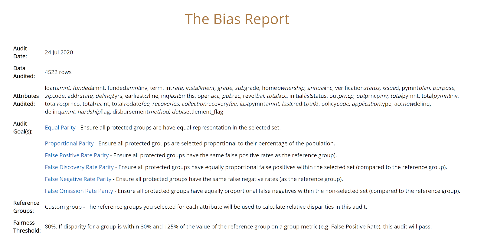
The report has a fixed input format. It requires:

• Score: The model predictions. This column can be either class probabilities, or even class itself.
• Label: This is the ground truth value of the data. This column represents the actual true labels.
• Attribute(s): These columns are the data. All the features, be it category, continuous fall under these columns.

Following is sample for the report format:

A sample report can be found here. The report can be mainly divided into 3 parts.

1. Summary of the metrics,
2. The relative values of metrics with reference to the protected variable.
3. The absolute values of metrics with reference to the protected variable.

Fairness Metrics

This tutorial heavily depends on metrics like accuracy, parity difference, equal odds difference, disparate impact, theil index, and other. So it's better to have a good understanding for the same. Let's look at them now. Refer to this wikipedia page for more information.

Equal Parity

Ensure all protected groups have equal representation in the selected set. This criteria considers an attribute to have equal parity if every group is equally represented in the selected set. In simple terms, it tells about the data's distribution among the categories.

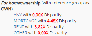
For example, consider the column ‘homeownership' from our Lending Club data. The available categories are [‘Any', ‘MORTGAGE', ‘RENT', ‘OTHER']. We see that there is unequal distribution of them in the data.

Proportional Parity

Ensure all protected groups are selected proportional to their percentage of the population. This criteria considers an attribute to have proportional parity if every group is represented proportionally to their share of the population. If your desired outcome is to intervene proportionally on people from all categories, then you care about this criteria

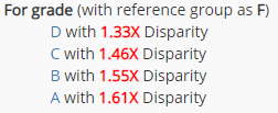
For example, the disparity for ‘Grade' is

False Positive Rate Parity

Ensure all protected groups have the same false positive rates (as the reference group). This criteria considers an attribute to have False Positive parity if every group has the same False Positive Error Rate.

For example, the FPR for column ‘homeownership' is

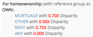
This means that categories with ‘Mortgage' have 0.7 times the false positive rate as ‘Own' i.e. the model would predict positive class for ‘Own' more than the category ‘Mortgage'.

False Discovery Rate Parity

Ensure all protected groups have equally proportional false positives within the selected set (compared to the reference group). This criteria considers an attribute to have False Discovery Rate parity if every group has the same False Discovery Error Rate.

For example, again for homeownership, the FDR parity is

False Negative Rate Parity

Ensure all protected groups have the same false negative rates (as the reference group). This criteria considers an attribute to have False Negative parity if every group has the same False Negative Error Rate.

For example, for the column ‘term period' the FNR parity is

At the end of the report, the relative values and the absolute values for the metrics are reported.

Relative Value

Absolute Value

Different Point of View (POVs)

In this module we showcase how different people can read and/or analyze the report.

Let's start with a Data Scientist.

Data Scientist's POV

After reading the report, the data scientist would infer that the model is biased in many ways. Some of the possible scenarios to come up are as follows:

1. Looking at the Equal parity and Proportional parity metrics, she/he might want to reconsider the data itself. The data, itself, is biased against some categories and thus the model would be biased.

Solutions to this problem can be as follows:

1.Get more representative data. 2.Use stratify splitting to at least mitigate the proportional parity bias. 3.Assign instance weights or class weights to the different categories involved. 4.Have all the data on the same scale

2. Looking at the false positive/negative/discovery/omission rates, she/he might want to reconsider the model itself, or the hyperparameters for it.

Solutions to this problem can be addressed in following ways:

1.Experiment with different models like tree models, linear models or more try to add some form of non-linearity to the model thereby being able to capture the information. 2.Add high penalty for wrong classifications and reward. 3.Change the loss function. 4.Regularize the model by adding type I or type II penalty losses.

Finance Person's POV

Now, let's consider a finance person. Clearly, she/he doesn't have knowledge of the underlying model and cannot effectively change the model. Some of the possible scenarios for her/him would be as follows:

1. Looking at the favourable groups, she/he can form intuitions as to why the model would arrive at a certain decision. This would help them to answer any concerns that customers come up with.
2. Another understanding that they can develop looking at the favourable groups would be to apply extra scrutiny to them. Consider an applicant who falls under many favourable categories. This ‘favourableness' might compensate for the less favourable ones. The finance person can here check for those parameters and have more scrutiny for the same.
3. She/he can lower the threshold for the use case. Say, a score of >0.8 might result in positive class. They can reduce that score to, for example, >0.7 for an application that falls majorly in unfavourable class and increase the score to >0.85 for someone who is major favourable categories.

This way, one can ‘reject opinion' and ‘remove prejudice' from the model manually.

Dataset

Before we talk about dataset, it is important to know what can be considered as a protected variable.

Protected variable: An attribute that partitions a population into groups whose outcomes should have parity. Examples include race, gender, caste, and religion. Protected attributes are not universal, but are application specific.

For demonstration purposes, we are using 3 datasets:

• German credit data: The dataset's objective is to predict an individual's credit risk. Read more about the data here. Sex, privileged: Male, unprivileged: Female. Race, privileged: White, unprivileged: Not White.
• Adult dataset: The dataset's objective is to predict whether income exceeds $50K/yr based on census data. Read more about the data here. Sex, privileged: Male, unprivileged: Female. Race, privileged: White, unprivileged: Not White.
• Compas dataset: The dataset's objective is to predict a criminal defendant's likelihood of reoffending. Read more about the data here. Sex, privileged: Female, unprivileged: Male. Race, privileged: Caucasian, unprivileged: Not Caucasian.

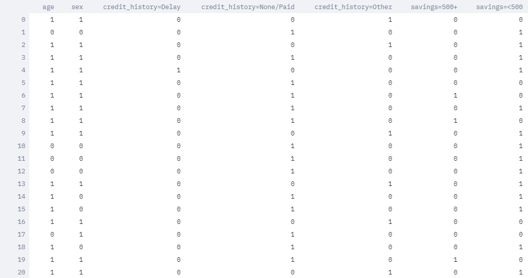
This is German data after cleaning and binning.

Methods

The methods can be broadly classified into 3 groups:

• Pre-processing methods
• In-processing methods
• Post-processing methods

Pre-Processing Methods

These techniques are applied before any training happens. In simple words, we play around with the data to mitigate the bias if any.

For example,

• Reweighing: This is a preprocessing technique that Weights the examples in each (group, label) combination differently to ensure fairness before classification
• Optimised Preprocessing: This is a preprocessing technique that learns a probabilistic transformation that edits the features and labels in the data with group fairness, individual distortion, and data fidelity constraints and objectives

In-processing methods

These techniques focus on the classifier itself. They add a regularisation term to the objective function of the classifier.

For example,

• Prejudice Remover: Prejudice remover is an in-processing technique that adds a discrimination-aware regularization term to the learning objective
• Adversarial Debiasing: Adversarial debiasing is an in-processing technique that learns a classifier to maximize prediction accuracy and simultaneously reduce an adversary's ability to determine the protected attribute from the predictions

Post-processing methods

These techniques are based on the predictions. These involve changing the predictions to make the classifier fairer.

For example,

• Reject Opinion: Reject option classification is a postprocessing technique that gives favorable outcomes to unprivileged groups and unfavorable outcomes to privileged groups in a confidence band around the decision boundary with the highest uncertainty
• Equal Odds: Equalized odds postprocessing is a post-processing technique that solves a linear program to find probabilities with which to change output labels to optimize equalized odds.

We showcase following methods:

• Reweighing (pre-processing)
• Prejudice Remover (in-processing)
• Adversarial Debiasing (in-processing)
• Reject Opinion (post-processing)

Fairness Metrics

This tutorial heavily depends on metrics like accuracy, parity difference, equal odds difference, disparate impact, theil index, and other. So it's better to have a good understanding for the same. Let's look at them now. Refer to this wikipedia page for more information.

Balanced Accuracy

Accuracy It is the ratio of number of correct predictions to the total number of input samples.Mathematically, it is defined as accuracy = correct predictions / total predictions

Statistical Parity Difference

Computed as the difference of the rate of favorable outcomes received by the unprivileged group to the privileged group. The ideal value of this metric is 0. Fairness for this metric is between -0.1 and 0.1

Equal Opportunity Difference

This metric is computed as the difference of true positive rates between the unprivileged and the privileged groups. The true positive rate is the ratio of true positives to the total number of actual positives for a given group. The ideal value is 0. A value of < 0 implies higher benefit for the privileged group and a value > 0 implies higher benefit for the unprivileged group. Fairness for this metric is between -0.1 and 0.1.

Average Odds Difference

Computed as average difference of false positive rate (false positives / negatives) and true positive rate (true positives / positives) between unprivileged and privileged groups. The ideal value of this metric is 0. A value of < 0 implies higher benefit for the privileged group and a value > 0 implies higher benefit for the unprivileged group. Fairness for this metric is between -0.1 and 0.1.

Disparate Impact

Computed as the ratio of rate of favorable outcome for the unprivileged group to that of the privileged group. The ideal value of this metric is 1.0 A value < 1 implies higher benefit for the privileged group and a value >1 implies a higher benefit for the unprivileged group. Fairness for this metric is between 0.8 and 1.2.

Theil Index

Computed as the generalized entropy of benefit for all individuals in the dataset, with alpha = 1. It measures the inequality in benefit allocation for individuals. A value of 0 implies perfect fairness. Fairness is indicated by lower scores, higher scores are problematic

Conclusion

This is the comparison between various methods using German Credit dataset with Sex as the protecte variable. The train column is the original column (without any mitigation of bias) and other columns are the various mitigation methods as discussed.

Following are some of the conclusions:

• Disparate Impact (DI): We can see that the initial DI was 0.64 which increased to higher values with different methods. This shows a positive effect of mitigating the losses.
• Theil Index: The lower the value, the more is the fairness. We can see that the index has much lower value for all the methods as compared to the original data.
• Another observation to make is regarding accuracy. We can see that the bias is decreasing but at the cost of accuracy. This is where the domain knowledge is needed to make a trade-off

1. Wikipedia for Fairness in ML
2. IBM's blog post