Description of the problem

An important application of predictive model is understanding sales. For manufacturers, having excess inventory can lead to additional warehouse storage costs, or outdated products. Having too little inventory can lead to lost sales and unmet demand. If a manufacturer can predict sales well before producing their products, they can meet their customer demands without wasting their resources.

In this problem, you will predict the monthly sales of the Hyundai Elantra car in the U.S. The Hyundai Motor Company is a major automobile manufacturer based in South Korea. The Elantra is a car model that has been produced by Hyundai since 1990 and is sold all over the world. We will build a linear regression model to predict monthly sales by using economic indicators of the United States as well as Google search queries. The data for this problem is contained in the file Elantra.csv, and can be found in the Online Companion. Each observation in the file is a month, from January 2010 to February 2014. You can also download the dataset using this link.

The variables are described in the table below.

What you will build

• Linear regression model

What you will learn

• Explore the data by using pandas and matplotlib
• Use normalization to preprocess the data
• Use linear regression to predict the value
• Evaluate the model by r^2 and Adjusted r^2

• pandas
• numpy
• matplotlib
• sklearn
• scipy
• statsmodels

First, use pandas pd.read_csv to read the csv file. Since the dataset doesn't have any invalid value, you can skip the step of cleaning the data.

Have a look of top 5 rows in the dataset:

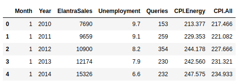
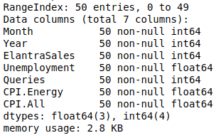
You can also use df.info() to get to know more about the data:

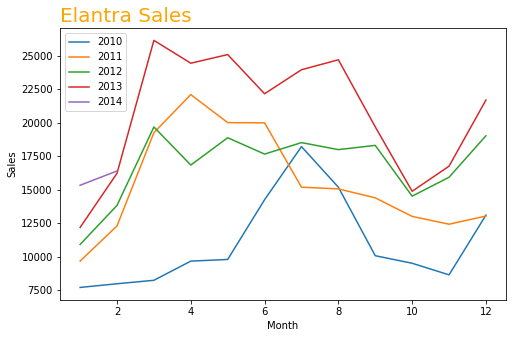
Set the "Month" column as the x-axis and " ElantraSales" as y-axis to visualize the data.

Start by splitting the dataset into a training set and testing set. The training set should have all observations for 2010, 2011 and 2012. The testing set should have all observations for 2013 and 2014.

Then, build a linear regression model to predict monthly Elantra sales (ElantraSales) using Unemployment, Queries, CPI.Energy, and CPI.All as the independent variables. Use the training set to build the model.

First, let us split the data into training and test set. Since the value in each variable have different range, you also need to scale the dataset. One simple way to do it is to use StandardScaler() in sklearn to create a standardization model.

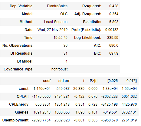
Then you can use sm.OLS() for the linear regression model, to train your model and get and evaluate the model.

The linear regression equation to predict ElantraSales:

The ANOVA shows r^2 score = 0.43 and Adjusted r^2 score = 0.35

A linear regression model is not always appropriate model for the data. One of the methods you can use to assess the appropriateness of the model is to define residuals and examining residual plots.

Residual= y test - y predicted value : The difference between the observed value of the dependent variable (y) and the predicted value (ŷ)

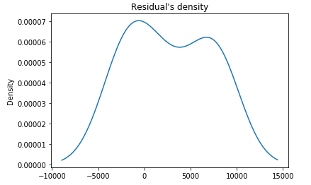
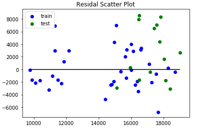
A linear model should have a normal distribution but in our plot, the residual is not normally distributed. To visualize the error of the prediction, we can try a residual scatter plot. If our model is good enough then the points should be randomly scattered around line zero.

We would like to improve our linear regression model by modeling seasonality. In predicting demand and sales, seasonality is often very important since demand tends to be periodic in time. For example, demand for jackets and coats tends to be higher in winter versus summer, while demand for sunscreen tends to be higher in the summer. We will incorporate seasonality into our model by using the Month variable.

Build a new linear regression model, this time using the Month variable as an additional independent variable. Again, use the training data to build your model.

The new linear regression equation with month variable added to predict ElantraSales:

r^2 score = 0.43 stays the same even after month feature added. Adjusted r^2 has decreased (0.34). This suggests that even variable is added, that does not improve a model.

Month variable should be a categorical variable rather than the numeric variables. Because we are not building a time series model and all the months should have the same weight to the model. To make Month as a categorical variable, we need to convert it (Month) into dummy/indicator variables.

Create a new linear regression model, this time with Month modeled as a categorical variable. You can do this by changing the values of Month to "January", "February", etc. or if you are using R, by converting Month to a factor variable.

Then you will get a series of dummy variables like this:

After cleaning the data, let us split the data and create a new regression model.

The linear regression equation to predict ElantraSales:

ANOVA shows r^2 score = 0.82:

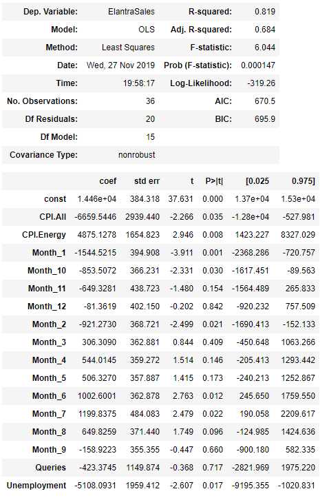
Compare the ANOVA from the one with month variable added as categorical values with the ones from the first and second regression equations. r^2 score (0.82) we have got here is much higher than the original scores. Is it a real improvement? Now, we can look at Adjusted r^2 score (0.68), which has also increased significantly. This means the model has become better.

Let us also look at p-value. Statistically, if the p-value is 0.05 or smaller at a significance level of 5%, the variable is significant. From the ANOVA above, following variables, CPI.All, CPI.Energy, Month_1, Month_10, Month_2, Month_6, Month_7 and Unemployment are statistically significant.

Now, let us move forward with the regression model with month variable added as categorical variables and try on the test set. r^2 score = 0.35 is not much high as you would have expected, but you can see some improvement in the model based on the plots below. Residual density plot is almost normally distributed, and Residual is more scattered around 0.

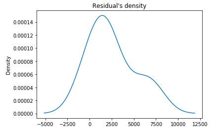
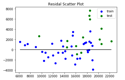
As shown above, the model fits training data very well in terms of r^2 and statistical hypothesis testing, but it poorly performs on the test data. This is a classical overfitting case. The following two ideas may help you solve the issue.

One potential approach is to reduce the number of features; we have a number of variables for the month feature (Jan through Dec), and you may have noticed that the values of coefficients for March through August is positive, while the values for the rest is negative. We could only add one indicator variable by distinguishing month variables into two groups, negative and positive, so that the number of features will be reduced. Another approach is adding a penalty factor into the cost function, such as using ridge regression to overcome the overfitting issue.

Bertsimas.D, O'Hair.A.K, Pulleyblank.W.R (2016) The Analytics Edge