Summary
Long short-term memory (LSTM) units (or blocks) are a building unit for layers of recurrent neural network (RNN). The expression long short-term refers to the fact that LSTM is a model for the short-term memory which can last for a long period of time. An LSTM is well-suited to classify, process and predict time series given time lags of unknown size and duration between important events. LSTMs were developed to deal with the exploding and vanishing gradient problem when training traditional RNNs. Relative insensitivity to gap length gives an advantage to LSTM over alternative RNNs, hidden Markov models and other sequence learning methods in numerous applications.
In this project, we use LSTM model to predict the weather. The weather data is from 09/01/2015 to 09/30/2015 collected from http://www.ncdc.noaa.gov/qclcd/QCLCD.
- tensorflow
- pymongo
- datetime
- numpy
- pandas
- bson
- sklearn
- seaborn
- lstm (lstm.py script in the directory)
- data_processing (data_processing.py script in the directory)
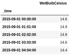
First, use pandas pd.read_csv to read the excel file and have a look of top 5 rows in the dataset (part of the columns):

The original data has 44 features, where 15 numeric variables and 29 categorical variables. In this project, we will only use "WetBulbCelsius" to make LSTM prediction.
Before the prediction, let us have a look at other features.
You can plot a density distribution plot to see the difference between "WetBulbCelsius" and "DryBulbCelsius". The plot should be like this:
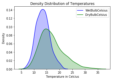
From the plot, you can learn that generally, the dry bulb temperatures are higher than the wet bulb temperatures and most wet bulb temperatures are in range 10 to 20.
Is there any correlations between other features?
Try to draw scatter plots for joint relations and histograms for univariate distributions.
Features ['Date', 'Visibility', 'DryBulbCelsius', 'WetBulbCelsius', 'RelativeHumidity', 'WindSpeed', 'RecordType', 'HourlyPrecip' ]
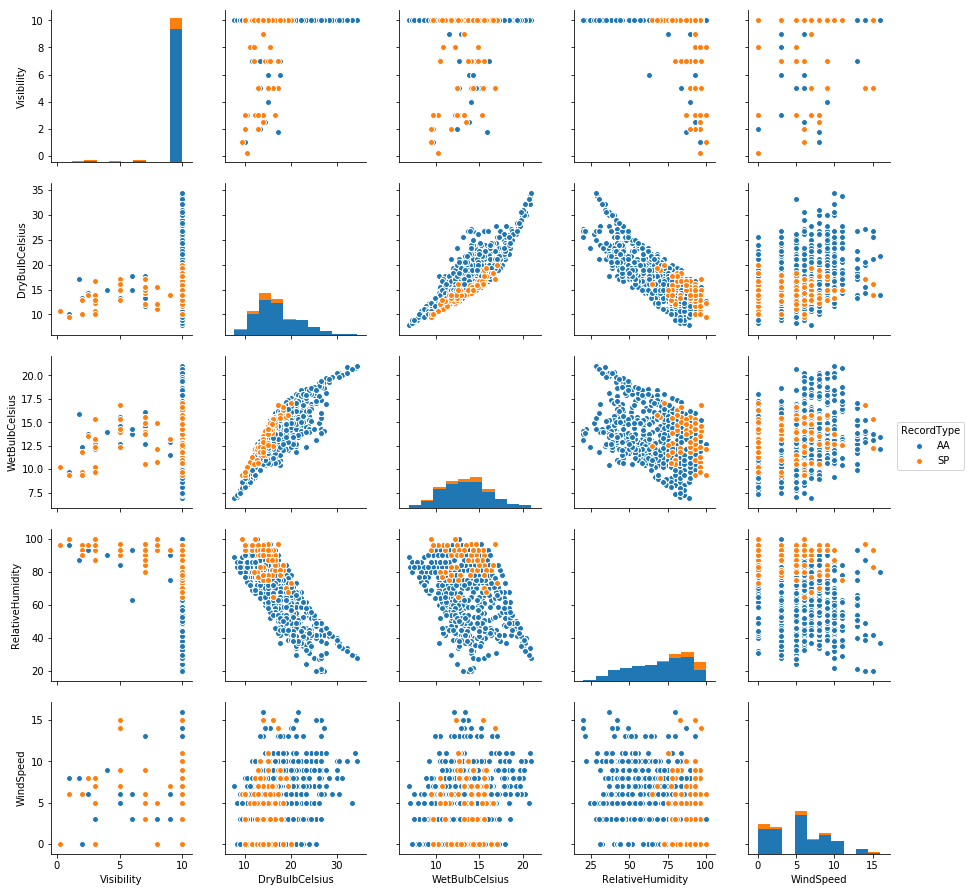
It is not hard to see that wet bulb temperature has a high correlation with dry bulb temperature and relative humidity.
Now, you need to preprocess the dataset for the following modeling. Scale values to reasonable values and convert to float. Keep the "WetBulbCelsius" column and convert the "Date", "Time" columns into a time-series column "_time"
The weather data should be like this:
You can also draw a time-series plot to see the change of temperatures.
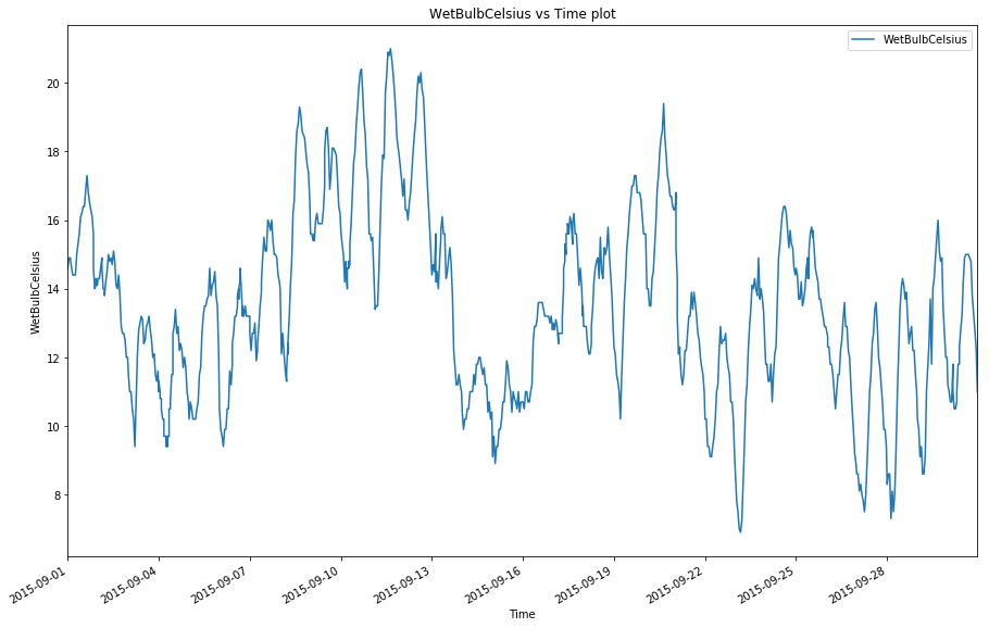
The plot shows a periodical temperature change in a month. This is a good sign for your time-series prediction model.
Before pre-processing and modeling, you need to set up the hyperparameter. The hyperparameters below is the one we defined at the beginning of the project.
LOG_DIR = './ops_logs/lstm_weather'
TIMESTEPS = 10
RNN_LAYERS = [{'num_units': 5}]
DENSE_LAYERS = [10, 10]
TRAINING_STEPS = 100000
BATCH_SIZE = 100
PRINT_STEPS = TRAINING_STEPS / 100
You can use functions in data_processing.py to split the data directly. It splits the data into 10% testing set, 10% validation set, 80% training set and stores them in a two dictionaries, one for features, one for target.
Now you can build the Long term short memory model (LTSM) with the hyperparameters defined above.
regressor = learn.SKCompat(learn.Estimator(
    model_fn=lstm_model(
        TIMESTEPS,
        RNN_LAYERS,
        DENSE_LAYERS
    ),
    model_dir=LOG_DIR
))
lstm_model is the deep model defined in lstm.py script.
Then, create a LSTM instance and validation monitor to train the model.
# create a lstm instance and validation monitor
validation_monitor = learn.monitors.ValidationMonitor(X['val'], y['val'],
                                                     every_n_steps=PRINT_STEPS,
                                                     early_stopping_rounds=1000)
regressor.fit(X['train'], y['train'],
              monitors=[validation_monitor],
              batch_size=BATCH_SIZE,
              steps=TRAINING_STEPS)
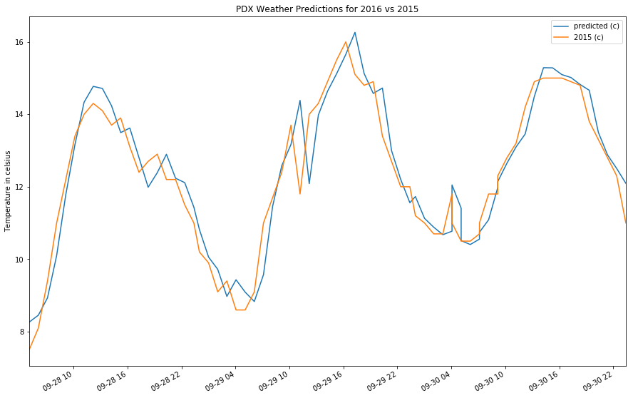
We use mean squared error metrics from sklearn to evaluate the model. The result shows the mean squared error is 0.43866. Not bad, right?
To have a better idea of the prediction from the model, you can plot the prediction with their true value.
https://github.com/mouradmourafiq/tensorflow-lstm-regression