Last Updated: 06/04/2020
What is a Generative Adversarial Network (GAN)?
A generative adversarial network (GAN) is a class of machine learning frameworks invented by Ian Goodfellow and his colleagues in 2014. Two neural networks contesting with each other in a zero-sum (or a min-max) game. Given a training set, this technique learns to generate new data with the same statistics as the training set.
If such a model is trained on, for example, time-series data of the Vix dataset, it should be able to generate good quality data for the Vix dataset.
Use Case
We use GAN for Univariate time series forecasting.
What will you build?
- A Generative Adversarial Network for generating synthetic univariate time series data.
What will you learn?
- Preprocessing required for the generation of synthetic time series
- How to make GAN model
- How to analyze various generated scenarios
Example Request:
- Get the Simulated data from given data set
POST /gan/simulation?model_name=demo_trail&size=1000&length=15&version=1.0&access_token=xxx
Host: https://gan.quantuniversity.com
Authorization: xxxxx
Content-Type: application/json
connection: keep-alive
content-length: 322241
content-type: application/json
date: Mon,19 Jul 2021 18:28:05 GMT
server: nginx/1.14.0 (Ubuntu)
Accept-Charset:utf-8
The definition of request is equal to the regular call to a post above. The response is identical except for adding four additional fields
Fields | Type | Description |
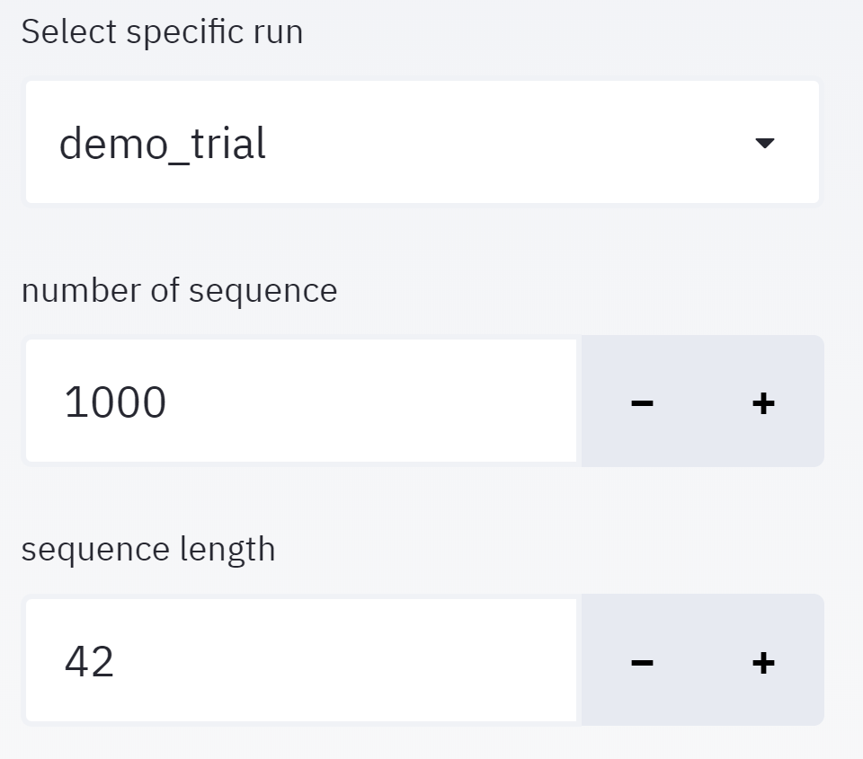
model_name | string | Select which dataset you have uploaded. For the current service, we only support the Vix model |
size | int | It specifies the number of simulations you want to generate |
length | int | It defines the forecast period. It specifies how much in the future you want to forecast |
version | float | It indicates the version you are using |
There are additional rules around publishing that each request to this API must respect:
- You should get access_token from QuUniversity and use that token to query every APIs it provides. Please the link: https://academy.qusandbox.com
Problems errors:
Error code | Description |
400 Bad Request | Required fields were invalid, not specified |
401 Unauthorized | The access_token is invalid or has been revoked |
422 Validation Error | The given parameter is invalid, please check the spelling |
500 Internal Server Error | Something went wrong on the model side |
|
|
This section includes an analysis of simulation data, and is divided into the following subsections:
- Simulation Samples
- Histogram/Distribution of observations at a single timestep, t (t=0 by default)
- Distributions of entire forecasting periods, represented by the mean and standard deviation
- K-Means Clustering of Scenarios
- Hierarchical Clustering of scenarios
- Clustering Comparison
- Discriminative Score(coming soon)
- Predictive Score(coming soon)
- PCA(coming soon)
- tSNE(coming soon)
Let's look at some of the plots. The plots are generated using the Vix dataset.
Simulation Samples
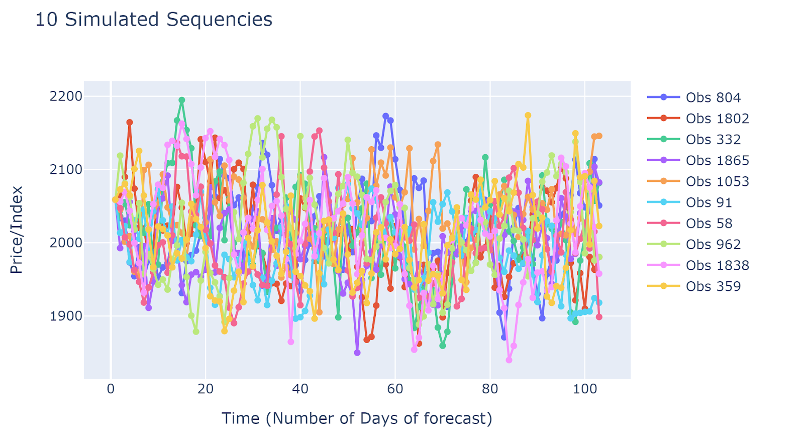
Simulated results are quite different from each other. This implied that the simulation results may capture many different scenarios. The disadvantage would be due to a large number of simulated sequences, it is hard to have generalized insights.
Histogram/Distribution of observations at a single timestep
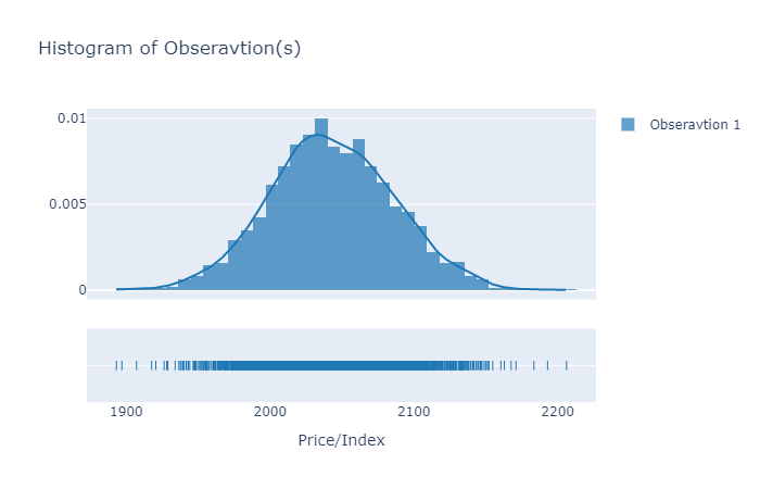
It is recommended to plot the histogram of the first time point. If it is distributed around the latest realized value (prices/index), then at least we can say that simulated data is not unrealistic.
K-Means Clustering of Scenarios
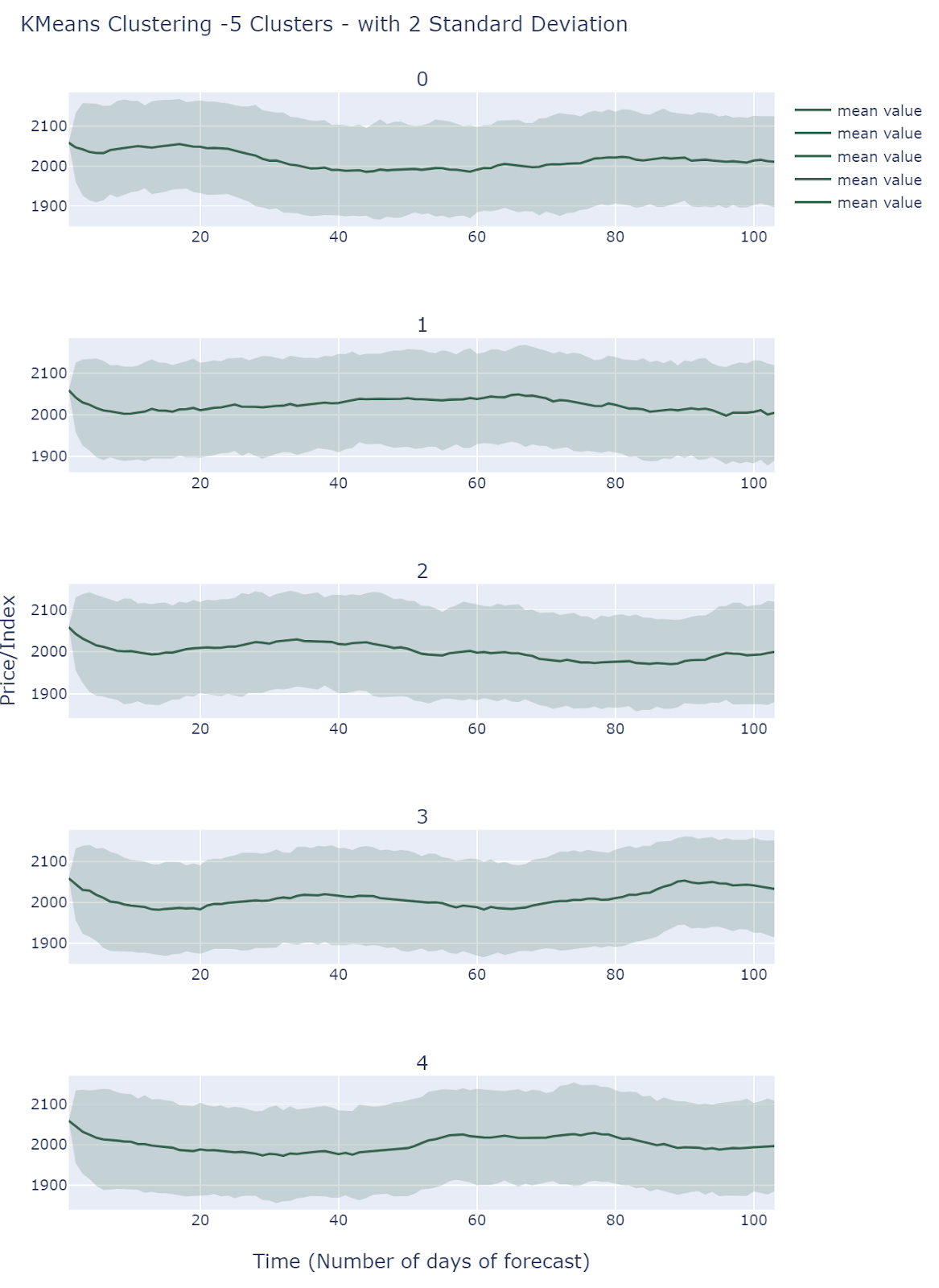
By default, we choose 5 clusters using L2-K-Means clustering to extract different scenarios.
All Clusters behave differently and they all fall into comparable ranges. Simulations do show different scenarios but it is still unclear how to interpret these results.
Hierarchical Clustering of scenarios
By default, we choose 5 clusters using Hierarchical Clustering(KL Divergence Affinity) to extract different scenarios. Cluster 0 and 1 presents relatively low volatilities, and cluster 2 and 3 shows medium volatilities. Cluster 4 is the most volatile one among all clusters. Therefore, the Hierarchical Clustering method groups observations based on volatility.

Clustering Comparison
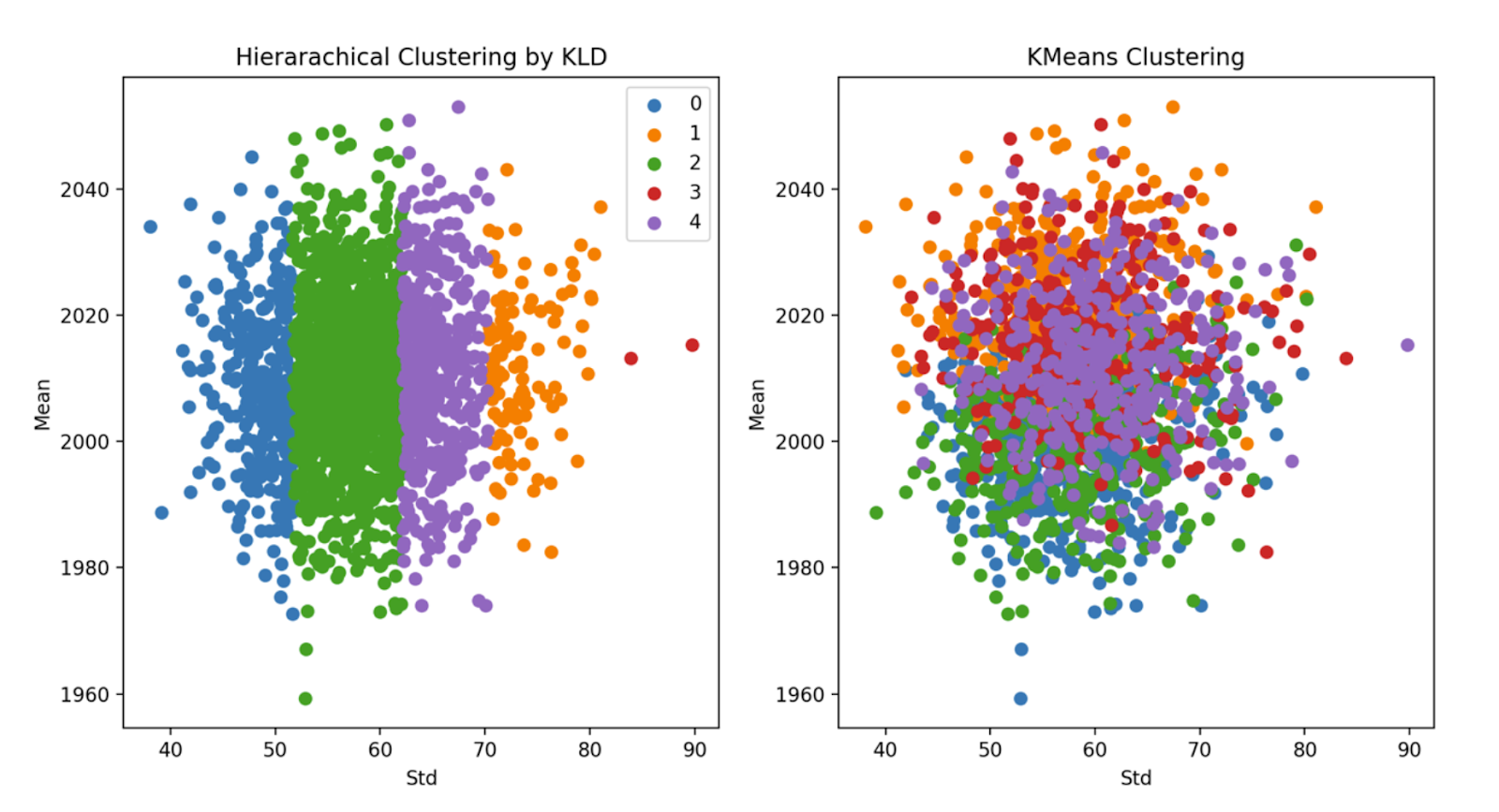
It is impossible and meaningless to analyze each sequence of simulated Prices. Instead, we should focus on some 'major' pattern reflected by the simulated data. In order to capture the 'major' pattern from simulation results, KMeans(L2 distance) and Hierarchical Clustering(KL Divergence Affinity) are applied, and Line Area charts would be implemented for each cluster.
Each cluster could be regarded as a potential scenario for Price. If viewed this way, further scenario analysis could be done for different clusters, which may lead to robust decision-making.
