Generative Adversarial Network

Last Updated: 06/04/2020

What is a Generative Adversarial Network (GAN)?

A generative adversarial network (GAN) is a class of machine learning frameworks invented by Ian Goodfellow and his colleagues in 2014. Two neural networks contest with each other in a zero-sum (or a min-max) game . Given a training set, this technique learns to generate new data with the same statistics as the training set.

If such a model is trained on, for example, time series data of Apple's stock price, it should be able to generate, atleast, good quality data for Apple's stock price. Whereas the same model won't be able to generate, Microsoft's price.

After training, we can generate data by simply noise into the model.

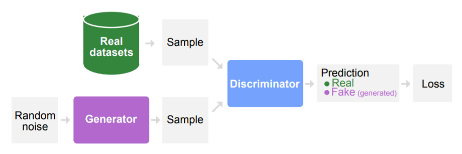
As seen from the figure, the input to the generator model is noise. It generates a fake sample and then discriminator distinguishes between real data and generated (or fake) data.

Use Case

We use GAN for Univariate time series forecasting.

What will you build?

A Generative Adversarial Network for generating synthetic univariate time series data.

What will you learn?

Preprocessing required for generation of synthetic time series
How to make GAN model
How to analyse various generated scenarios

Getting Data

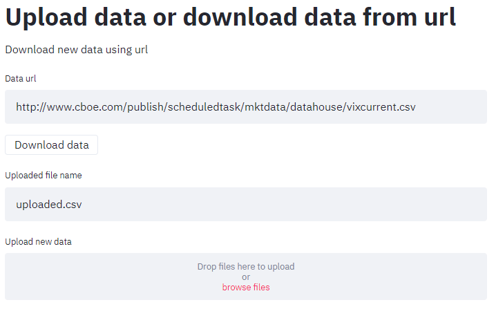
We can fetch the data in 2 possible ways:

By specifying a data URL
Uploading .csv file

The data should has values (prices, indexes etc.) and corresponding timestamp.

Restructuring data for ingestion

Since we are dealing with time series data, data values might show some increasing/decreasing trends. In other words, they might not fall on the same scale. So, it is necessary to normalise the dataset.

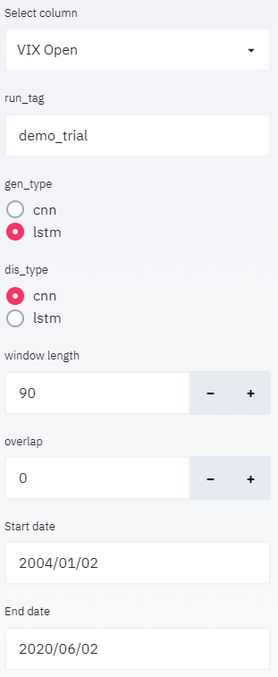
The preprocessing function normalises the value. Apart from this, it also provides functionality for clipping the data between start_date and end_date. You can also specify the window and overlap periods for restructuring the data. In other words, you can restructure your 1-dimensional data into N sequences of window length with overlap days.

You can select a column from the dataset available.
Run Tag is a name placeholder for the experiment being conducted.
Generator type (gen_type) and Discriminator type (dis_type) allows you to choose the underlying model architecture for the experiment.
Window Length specifies how long the sequence should be i.e. how many days' of data should 1 sequence have. Whereas, overlap specifies how much each sequence should overlap
For example, your data is . A window length of, say 10, and overlap length of, say 0, would result in following restructured data: Sequence 1: Sequence 2: and so on.
A window length of, say 10, and overlap length of, say 5, would result in following restructured data: Sequence 1: Sequence 2: and so on.
Start and End date can be used to clip the dataset as per the usage.

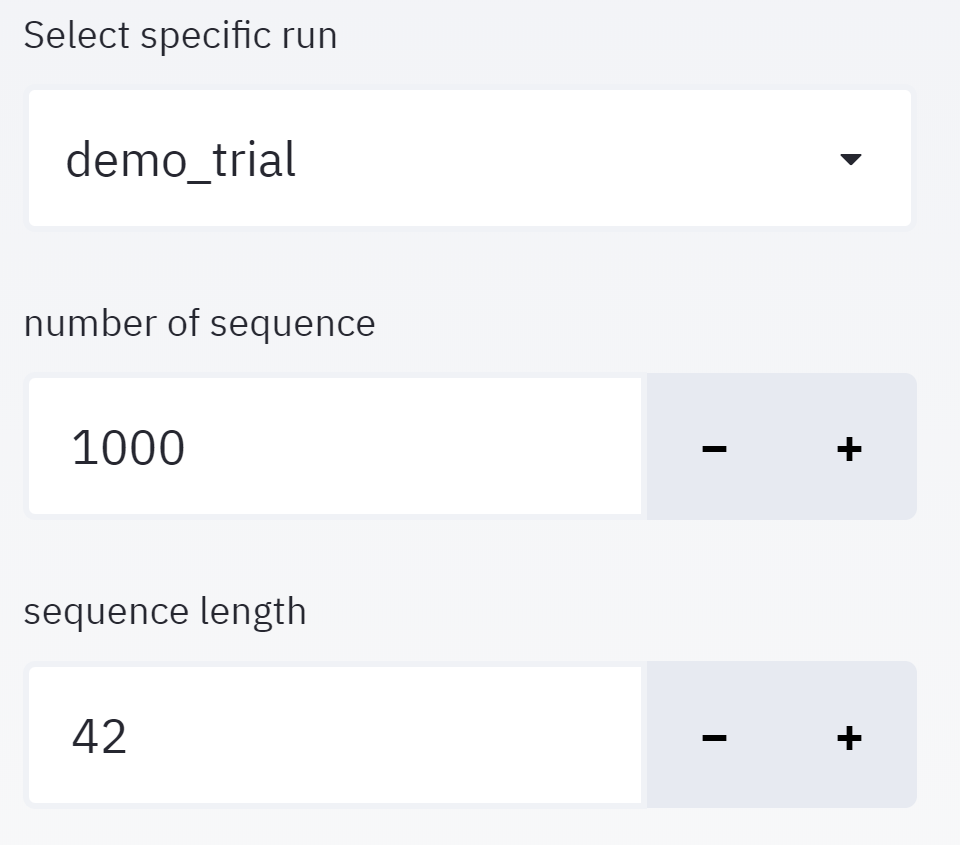
Here you can define a basic model parameter.

Epochs specify how many passes should the model make over the dataset for learning. For faster training, the default value is set to 20.

Start training button would initialise the model and begin training.

About model

The model comprises a generator and discriminator model. As the name suggests, the generator is responsible for generating data whereas discriminator distinguishes between generated (fake) and real data.

The generator model takes a fixed-length random vector as input and generates a sample in the domain. The vector is drawn randomly from a Gaussian distribution, and the vector is used to seed the generative process. After training, points in this multidimensional vector space will correspond to points in the problem domain, forming a compressed representation of the data distribution or latent space. The generator model applies meaning to points in a chosen latent space, such that new points drawn from the latent space can be provided to the generator model as input and used to generate new and different output examples.

The discriminator model takes an example from the domain as input (real or generated) and predicts a binary class label of real or fake (generated). The real example comes from the training dataset. The generated examples are output by the generator model. The discriminator is a normal classification model.

The two models, the generator and discriminator, are trained together. The generator generates a batch of samples, and these, along with real examples from the domain, are provided to the discriminator and classified as real or fake. The discriminator is then updated to get better at discriminating between real and fake samples in the next round, and importantly, the generator is updated based on how well, or not, the generated samples fooled the discriminator. In this way, the two models are competing against each other, they are adversarial in the game theory sense, and are playing a zero-sum game.

After the training process, the discriminator model is discarded as we are interested in the generator.

You can select which model to run based on the name tag you mentioned in the previous step.
Number of sequences specify the number of simulations you want to generate.
Sequence length defines the forecast period. It specifies how much in future you want to forecast. (The maximum value can be the window length that you specified in the train module)

This section includes analysis over simulation data, and divided into the following subsections:

Simulation Samples
Histogram/Distribution of observations at a single timestep, t (t=0 by default)
Distributions of entire forecasting periods, represented by mean and standard deviation
K-Means Clustering of Scenarios
Hierarchical Clustering of scenarios
Clustering Comparison
Discriminative Score(coming soon)
Predictive Score(coming soon)
PCA(coming soon)
tSNE(coming soon)

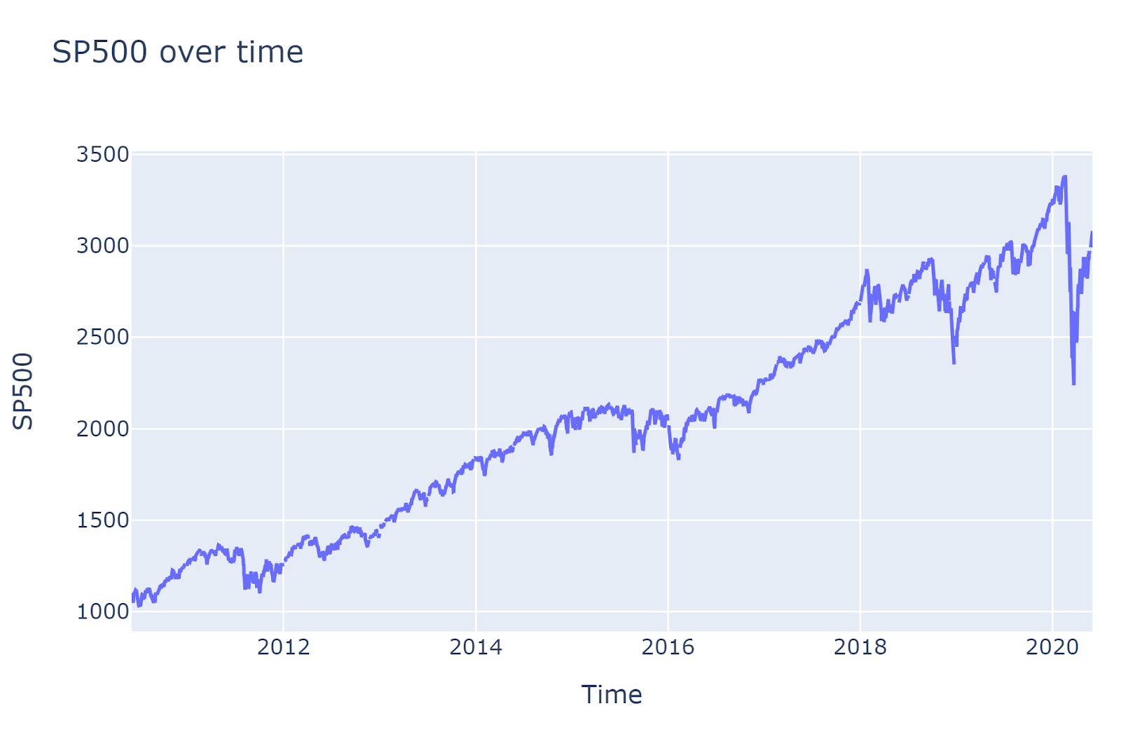
Let's look at some of the plots. The plots are generated using the S & P 500 index.

Note: The training date period is 2014.

Simulation Samples

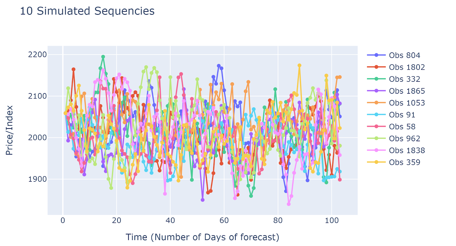
Simulated results are quite different from each other. This implied that the simulation results may capture many different scenarios. The disadvantage would be due to the large number of simulated sequences, it is hard to have generalized insights.

Histogram/Distribution of observations at a single timestep

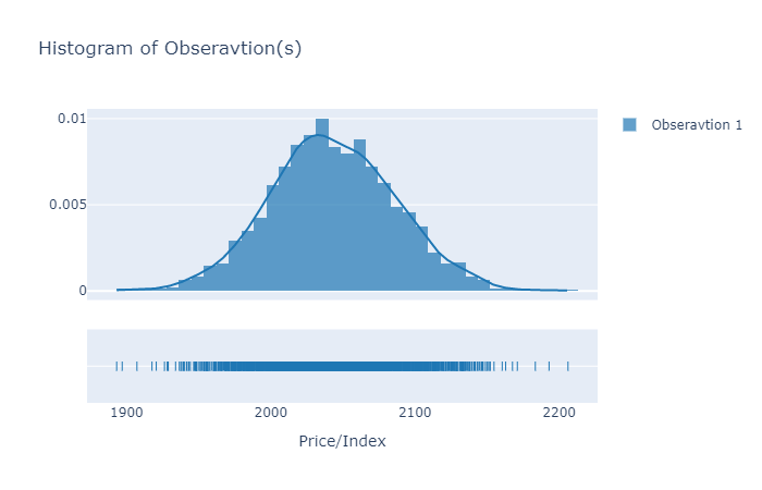
It is recommended to plot the histogram of the first time point. If it is distributed around the latest realized value (prices/index), then at least we can say that simulated data is not unrealistic.

K-Means Clustering of Scenarios

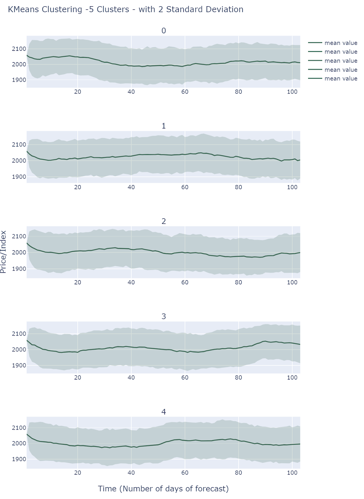
By default , we choose 5 clusters using L2-K-Means clustering to extract different scenarios.

All Clusters behave differently and they all fall into comparable ranges. Simulations does show different scenarios but it is still unclear how to interpret these results.

Hierarchical Clustering of scenarios

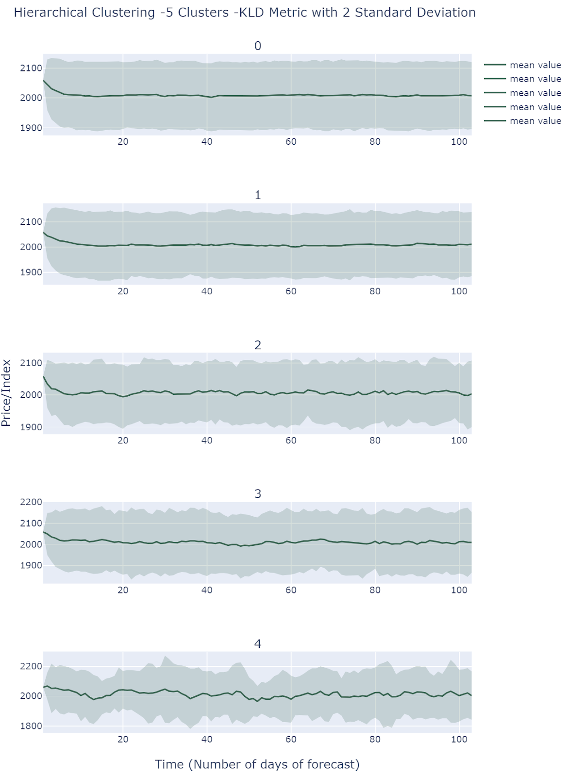
By default , we choose 5 clusters using Hierarchical Clustering(KL Divergence Affinity) to extract different scenarios. Cluster 0 and 1 presents relatively low volatilities, and cluster 2 and 3 shows medium volatilities. Cluster 4 is the most volatile one among all clusters. Therefore, Hierarchical Clustering method groups observations based on volatility.

Clustering Comparison

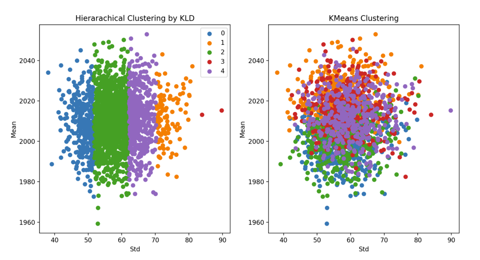
It is impossible and meaningless to analyze each sequence of simulated Price. Instead, we should focus on some 'major' pattern reflected by the simulated data. In order to capture the 'major' pattern from simulation results, KMeans(L2 distance) and Hierarchical Clustering(KL Divergence Affinity) are applied, and Line Area charts would be implemented for each cluster.

Each cluster could be regarded as a potential scenario for Price. If viewed this way, further scenario analysis could be done for different clusters, which may lead to robust decision making.