Description of the problem
Many people struggle to get loans due to insufficient or non-existent credit histories. And, unfortunately, this population is often taken advantage of by untrustworthy lenders.
Home Credit strives to broaden financial inclusion for the unbanked population by providing a positive and safe borrowing experience. In order to make sure this underserved population has a positive loan experience, Home Credit makes use of a variety of alternative data-- including telco and transactional information-- to predict their clients' repayment abilities.
What you will build
- Logistic regression classifier
- Random forest classifier
- Gradient boosting classifier
What you will learn
- Perform exploratory data analysis (EDA) on data
- Clean large dataset to fit the model
- Use models in sklearn to build and train data, and evaluate their performance
- pandas
- numpy
- matplotlib
- seaborn
- sklearn
In this project, you will use two datasets: HomeCredit_columns_description.csv and application_train.csv.
First, take a look at the main dataset.


The dataset is almost 300MB with 307,510 rows and 122 columns. Most variables are numeric and there are also 16 categorical variables. It is all the information about each loan application at Home Credit. Every loan has its own row and is identified by the feature SK_ID_CURR. The TARGET indicates 0: the loan was repaid, or 1: the loan was not repaid. Below is the description of dataset.
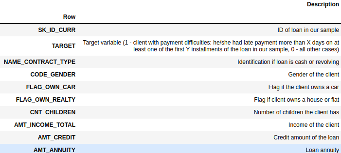 .
.
Examine the Distribution of the Target Column
The target variable is what you will predict: 0 indicates that the loan was repaid on time, or 1 indicates the client had payment difficulties.
Name | dtype | Description |
TARGET | object | Target variable (1 - client with payment difficulties: he/she had late payment more than X days on at least one of the first Y installments of the loan in our sample, 0 - all other cases) |
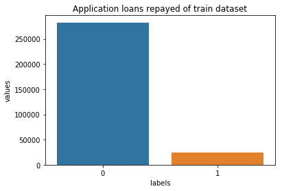
From this plot, you can see the data is imbalanced, the repaid cases is almost 9 times more than the unpaid cases. Downsampling or oversampling is recommended before fitting the model, which is explained later.
Examine the Distribution of the Other Columns
Name | dtype | Description |
NAME_CONTRACT_TYPE | object | Identification if loan is cash or revolving |
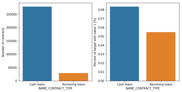
Contract type Revolving loans are just a small fraction (10%) from the total number of loans; however, when you focus on entries that had difficulties repaying, a much larger amount of Revolving loans is found.
Name | dtype | Description |
CODE_GENDER | object | Gender of the client |
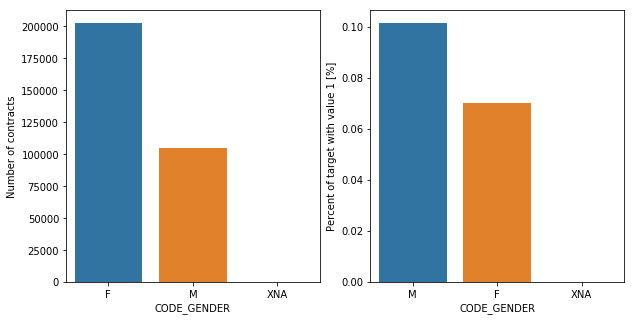
The number of female clients is almost double the number of male clients. Focusing on the entities with repayment difficulties, males have a higher chance of not being able to pay their loans back (9%) compared with females (7%).
Name | dtype | Description |
FLAG_OWN_CAR | object | Flag if the client owns a car |
FLAG_OWN_REALTY | object | Flag if client owns a house or flat |
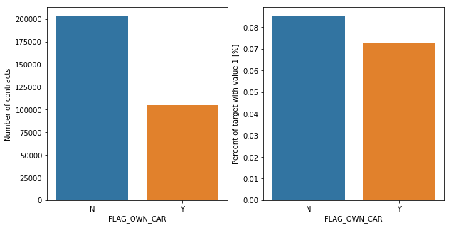
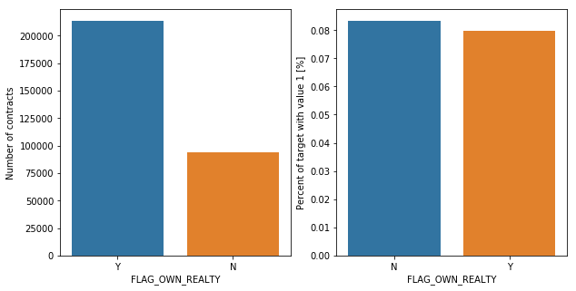
The graphs above were about car and realty ownership. Overall, there are twice as many clients who own realty, while half the number of clients own cars. Focusing on the entities unable to repay their loans, the percentage of those who own cars and those who do not is similar. In fact, with realty ownership, the percentage is almost the same. This suggests that car and realty ownership could be a big factor that influence on clients' inability of repayment.
Name | dtype | Description |
NAME_FAMILY_STATUS | object | Family status of the client |
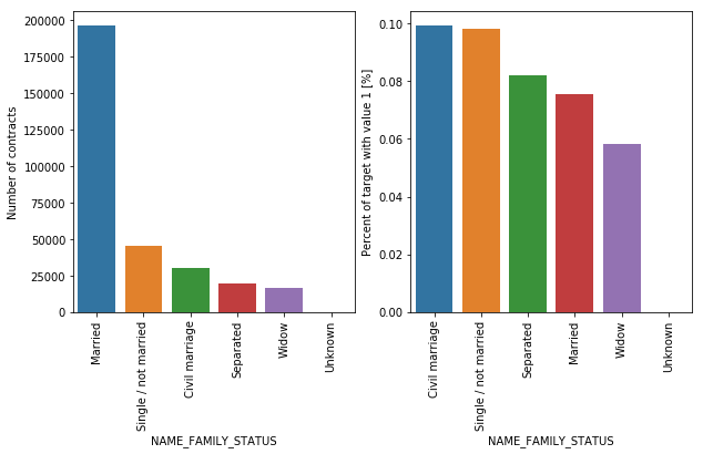
About 65% of the clients are married, followed by the clients with the status of single/not married and civil marriage. In terms of percentage of being unable to repay their loan, the three highest clients' status are civil marriage, single/not married and separated.
Name | dtype | Description |
CNT_CHILDREN | numeric | Number of children the client has |
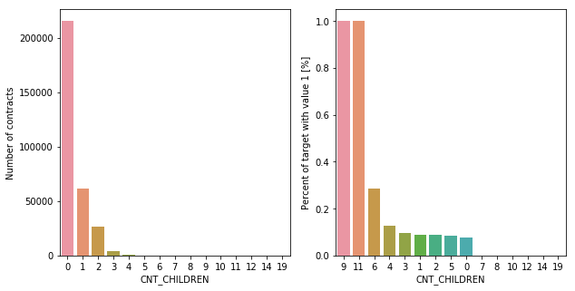
About 70% of the clients who take a loan have no children. The number of clients with a child is a quarter of the ones with no children, and the client number becomes drops with number of children increasing. As for the clients who are unable to repay their loans, there is about 10% of chance of not repaying if the have no or up to five children. If they have 9 or 11 children, there is almost no chance to pay their loans back.
Name | dtype | Description |
CNT_FAM_MEMBERS | numeric | How many family members clients have |
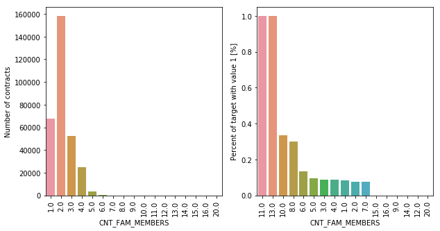
About 50% of the clients have 2 family members, followed by single persons (22%). As for the clients with inability to repay their loans, the percentage of an inability chance drops as the family number decreases.
Name | dtype | Description |
NAME_INCOME_TYPE | object | Clients income type (businessman, working, maternity leave,) |
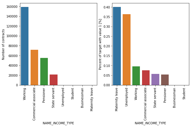
Half of the clients are working, followed by commercial associate (22%), pensioner (18%) and state servant (10%). For the group of enable to repay their loans, almost 40% is on maternity leave, followed by Unemployed (37%).
Name | dtype | Description |
OCCUPATION_TYPE | object | What kind of occupation does the client have |
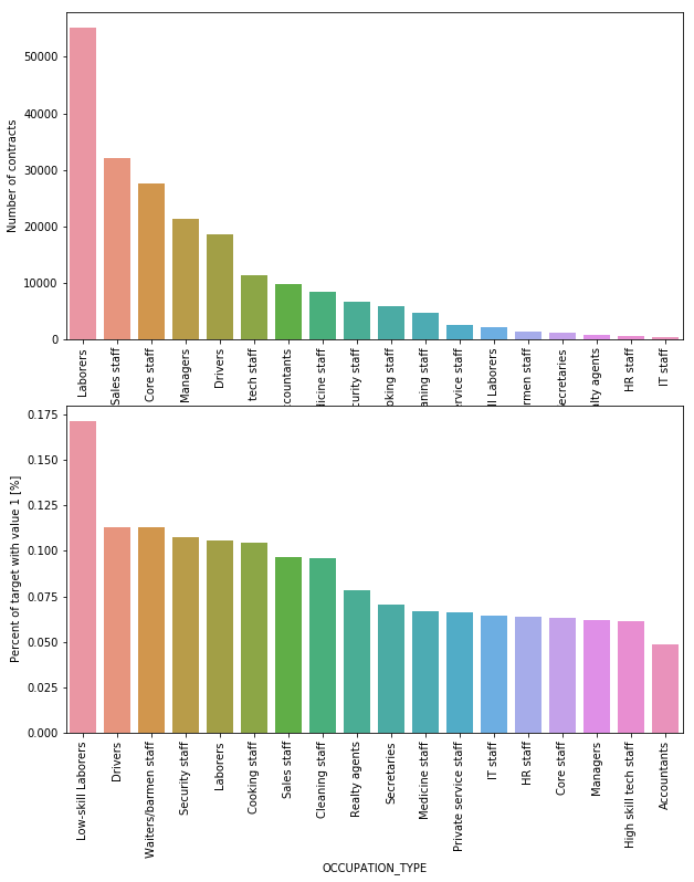
Laborers are the most popular occupation of all (20%), followed by Sales staff and Core stuff. IT staff are least likely to need loans. More than 17% of the clients with low-skilled occupations are unable to pay their loans, followed by Drivers and Waiters/barmen staff, Security staff, Laborers and Cooking staff.
Name | dtype | Description |
ORGANIZATION_TYPE | object | Type of organization where client works |
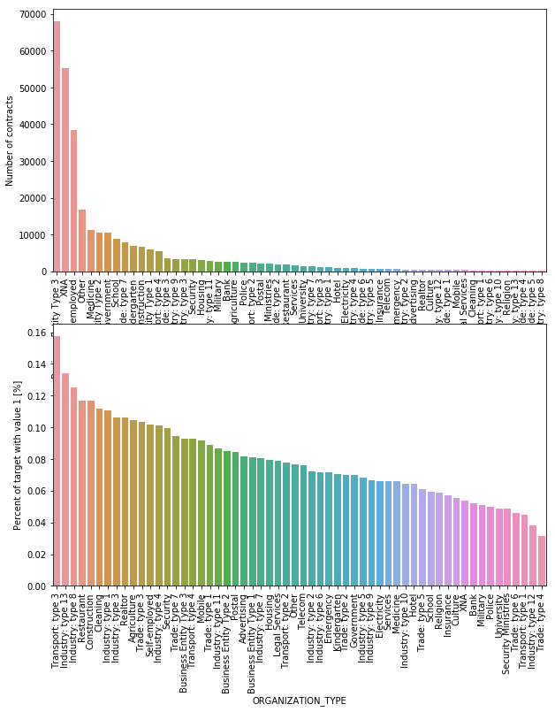
Organizations with highest percent of repayment inability are Transport: type 3 (16%), Industry: type 13 (13.5%), Industry: type 8 (12.5%), Restaurant and Construction (less than 12%).
Name | dtype | Description |
NAME_EDUCATION_TYPE | object | Level of highest education the client achieved |
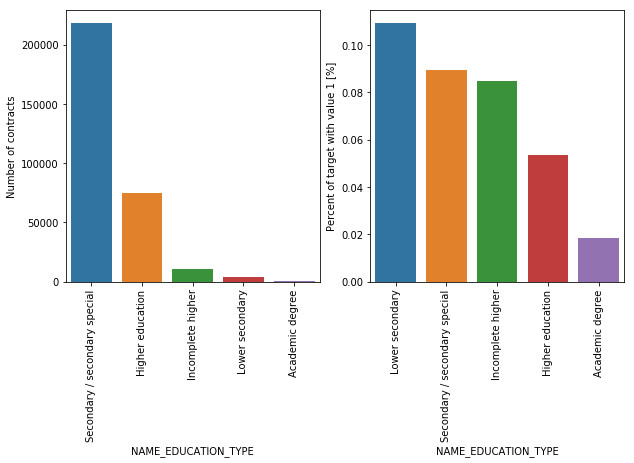
70% of the clients have Secondary / secondary special education, followed by clients with Higher education. Only a very small number of clients have their Academic degrees. More than 10% of clients who are unable to repay their loans have lower secondary education, followed by Secondary / secondary special, and incomplete higher. This may indicate that clients with lower education tend to have difficulty repaying their loans.
Name | dtype | Description |
NAME_HOUSING_TYPE | object | What is the housing situation of the client (renting, living with parents, ...) |
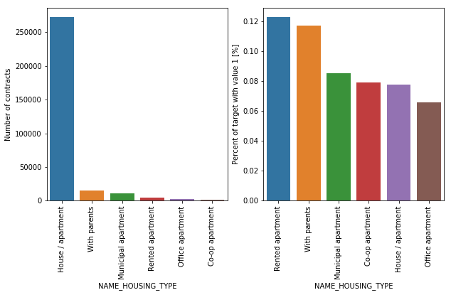
Over 250,000 applicants for credits registered their housing as House/apartment. Other categories have a very small number of clients (living with parents and Municipal apartments). From these categories, more clients who are unable to repay their loans live in a rented apartment or live with parents (more than 10%).
Name | dtype | Description |
DAYS_BIRTH | numeric | Client's age in days at the time of application |
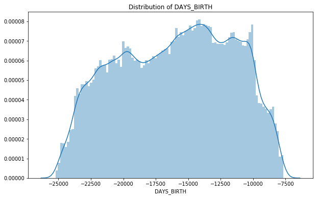
The value shows how many days have passed from the date of birth, where you can find the clients' age is between about 20 and 68 years. The highest peak of the distribution is between about 35 and 44 years old.
Name | dtype | Description |
DAYS_EMPLOYED | numeric | How many days before the application the person started current employment |
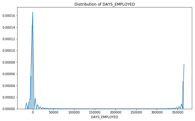
The negative values suggest the clients are unemployed. There is another peak after 350000, which does not make sense if the number is interpreted as days, which yields over 100. If we interpret the numbers by the minute, the number 350000 makes about 145 weeks (suppose a person worked 40 hours a week), which is about 2.7 years.
Name | dtype | Description |
DAYS_REGISTRATION | numeric | How many days before the application did client change his registration |
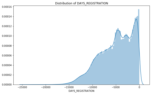
If clients changed their registration, some did so as old as 40 years ago. However, a lot of them changed their registration three years before their application, where you can see the highest peak.
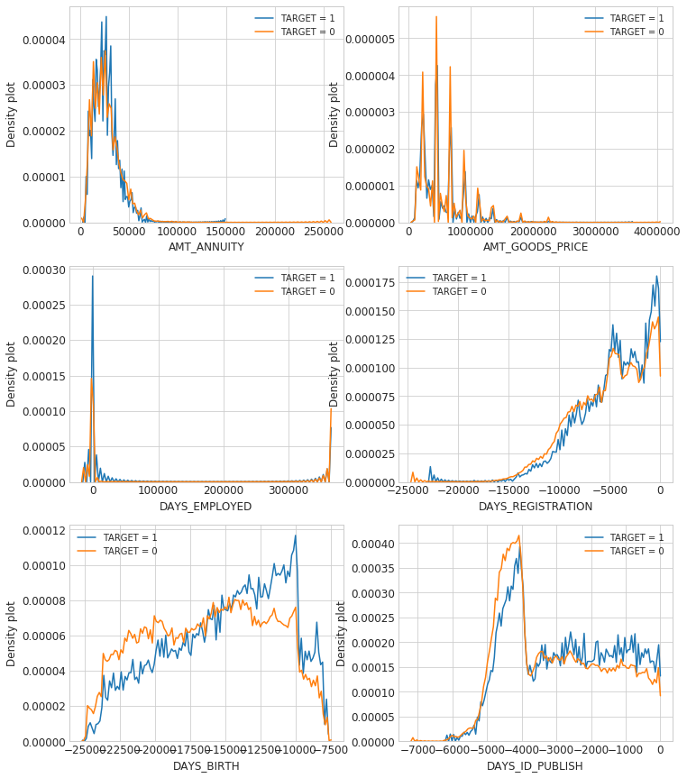
When you look at distribution charts with TARGET=1 and 0 at the same time, you can learn some characteristics of the features. The density plot for the clients who are not employed and unable to repay their loans is about twice as much as those who can pay. The density plot of the client with repayment inability is larger when they are young, which gradually decreases as they get older. The peak is when they are in their 20's, where the density is almost twice as large as the counterpart.
First, remove the columns where 40% percent or more of the variables are missing. We may also want to find columns that will not be significant for our model and remove them based on your exploratory analysis. We will remove EXT_SOURCE_2 and EXT_SOURCE_3 since the distribution graphs for Target=1 and Target=2 are normally distributed.
To deal with other missing values on numeric variables, you can use Pandas' fillna() function to fill in missing values in a dataframe. What would you fill the values with? You may need some strategies. In the notebook, we use three strategies.
- Replace all the Nan values with mean value of the column
- Replace all the Nan values with 0
- Replace all the Nan values with the most repeated value (mode) in that columns
Since there is no missing value in categorical variables, you can leave them as they are.
For categorical values, use LabelEncoder() to convert the categoricals values into machine-readable form.
Remove highly correlated predictors
Multicollinearity occurs when your model includes multiple factors that are correlated not just to your response variable, but also to each other. It may increase the standard errors of the coefficients which will make some variables statistically insignificant when they should not be significant. In order to select actual significant features, you may need to remove highly correlated predictors from the model.
After dropping highly correlated features, remember to convert the categorical variables into dummy variables.
In this project, we are going to use logistic regression classifier, random forest classifier and gradient boosting classifier in sklearn to predict the target.
Splitting data into train and test set
Split the data into 70% train set and 30% test set, separate the dependent and independent variables.
As we learned in the previous step, the TARGET value is unbalanced:

To handle the unbalanced dataset, you can try to up-sample minority class or down-sample majority class. In this notebook, we use the result of down-sampling.

Evaluate the model
The sklearn.metrics module implements several loss, score and utility function to measure classification performance. Some metrics might require probability estimates of the positive class, confidence values, or binary decisions values.
In this project, we use the following metrics:
- accuracy_score: Accuracy classification score
- classification_report: Computes precision, recall, and F1 scores
- roc_curve: Computes Receiver operating characteristic (ROC)
- roc_auc_score: Computes Area Under the Receiver Operating Characteristic Curve (ROC AUC) from prediction scores. The AUC score tells good balance (tradeoff) of true positive and false positive. The ideal AUC looks like a half moon in the graph.
Logistic Regression Classifier | |||
Accuracy score | 0.66 | Precision score | 0.59 |
Recall score | 0.66 | F1-score | 0.59 |
AUC | 0.53 |
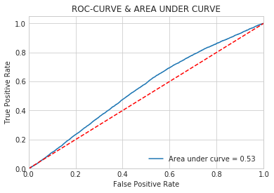
Random Forest Classifier | |||
Accuracy score | 0.66 | Precision score | 0.61 |
Recall score | 0.66 | F1-score | 0.59 |
AUC | 0.58 |
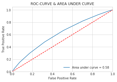
Gradient Boosting Classifier | |||
Accuracy score | 0.63 | Precision score | 0.63 |
Recall score | 0.63 | F1-score | 0.55 |
AUC | 0.63 |
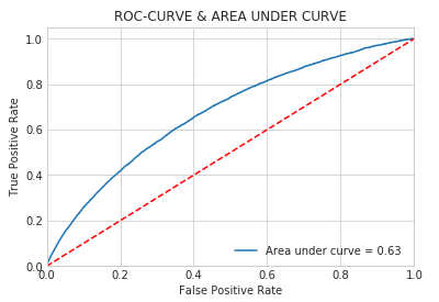
Result table

From the result, you can see that the Gradient Boosting Classifier has the best performance for this dataset based on the recall score (0.63) and AUC (0.63) However, the models have not been tuned and we only used the down-sampling data which would lose some information of the data. For further experiment, try to improve the performance of Gradient Boosting Classifier by yourself!
Kaggle. (2018) Home Credit Default Risk.