Last Updated: 06/03/2020
What is an Ornstein–Uhlenbeck (OU) Process?
The Ornstein–Uhlenbeck process is a stationary Gauss–Markov process, which means that it is a Gaussian process, a Markov process, and is temporally homogeneous.
Ornstein–Uhlenbeck Process model specification:

Ornstein–Uhlenbeck Process Parameter Estimation

Use Case
We use the OU process for Univariate time series forecasting.
What will you build?
- A OU Model for generating synthetic univariate time series data.
What will you learn?
- Preprocessing required for generation of synthetic time series
- How to make OU model
- How to analyse various generated scenarios
Getting Data
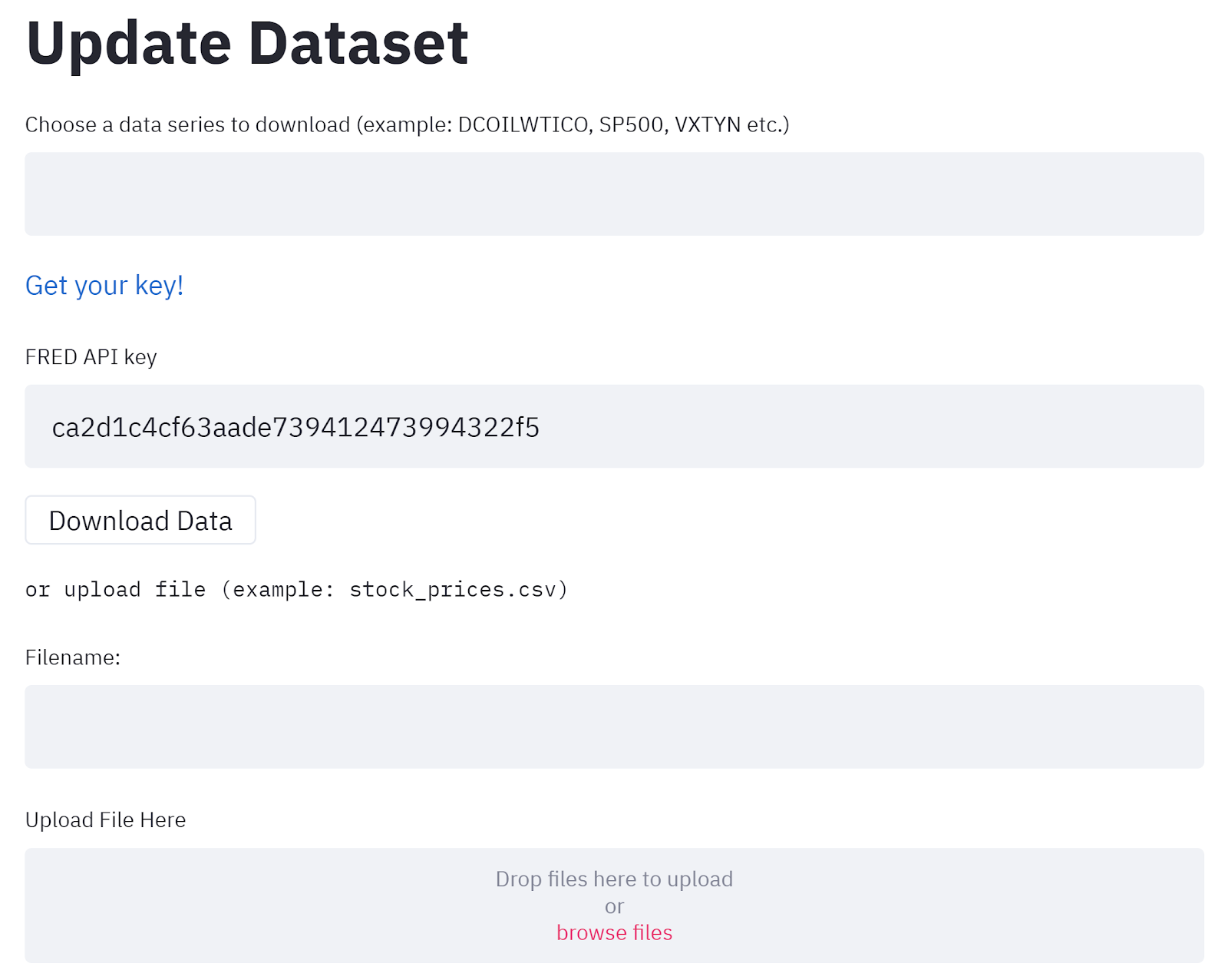
We can fetch the data in 2 possible ways:
- From FRED datasource (Learn more here)
- Uploading .csv file
The data has values (prices, indexes etc.) and corresponding timestamp.
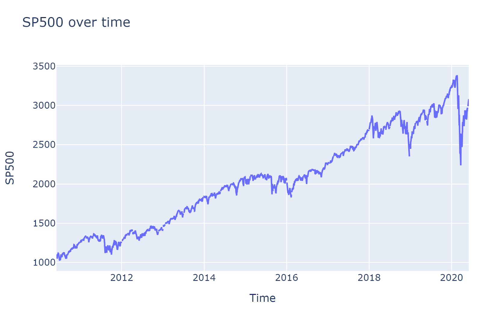
Restructuring data for ingestion
Since OU process assumes change of price is stationary, and price changes are not always stationary. It is necessary to convert price into log of price
The data is automatically converted from its original values  into returns
  .
.

Apart from this, this section also provides functionality for clipping the data between start_date and end_date.
| Training Start and End date can be used to clip the dataset as per the usage. Forecasting Horizon Forecast period specifies how much in future you want to forecast, determined by Start and End date. |
About model
The model does not have any hyper parameters to control. It is using log of price instead of return or price.
Model Result
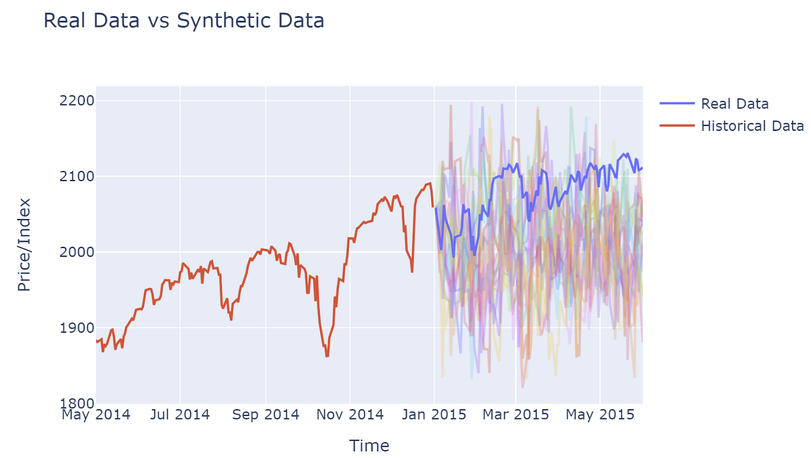
The graph of price, which is converted back from log of price, shows that simulations are very volatile and cannot easily find a noticeable pattern.
This section includes analysis over simulation data, and divided into the following subsections:
- Simulation Samples
- Histogram/Distribution of observations at a single timestep, t (t=0 by default)
- Distributions of entire forecasting periods, represented by mean and standard deviation
- K-Means Clustering of Scenarios
- Hierarchical Clustering of scenarios
- Clustering Comparison
- Discriminative Score(coming soon)
- Predictive Score(coming soon)
- PCA(coming soon)
- tSNE(coming soon)
| Simulations specify if you want to apply the following analysis over return or price. |
Simulation Samples
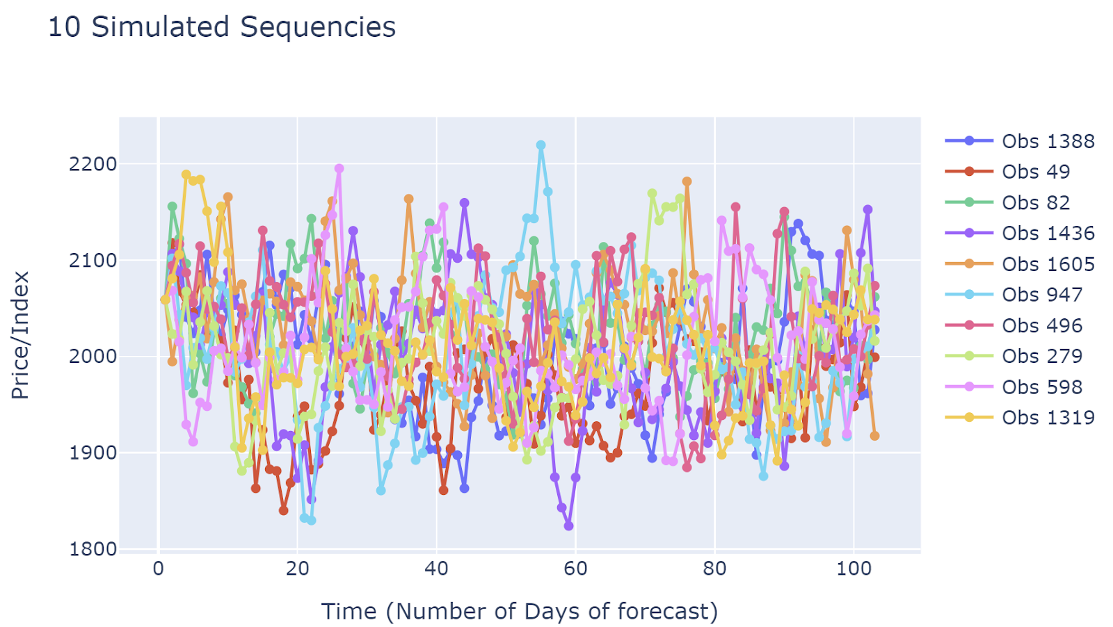
Take a look at some randomly selected simulations.Simulated results are quite different from each other. This implied that the simulation results may capture many different scenarios. The disadvantage would be due to the large number of simulated sequences, it is hard to have generalized insights.
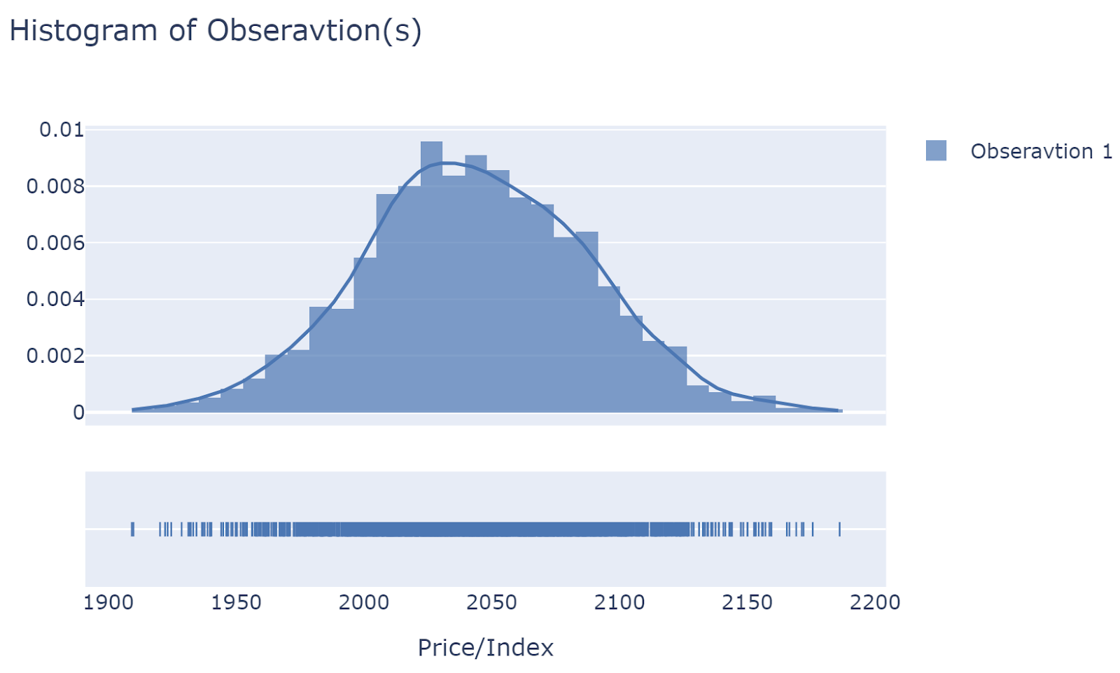
Histogram/Distribution of observations at a single timestep
It is recommended to plot the histogram of the first time point. If it is distributed around the latest realized value (prices/index), then at least we can say that simulated data is not unrealistic.
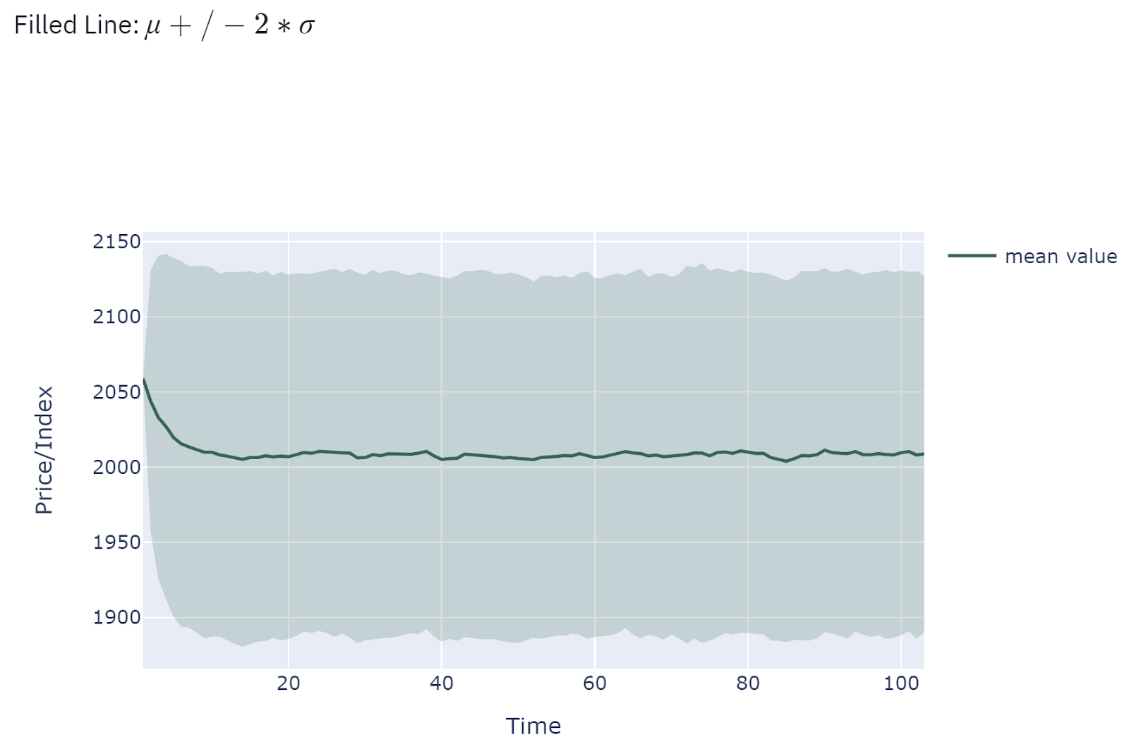
Distributions of entire forecasting periods
The middle line is the mean value of all simulations while the filled area is determined by the standard deviation of simulations at each time step.
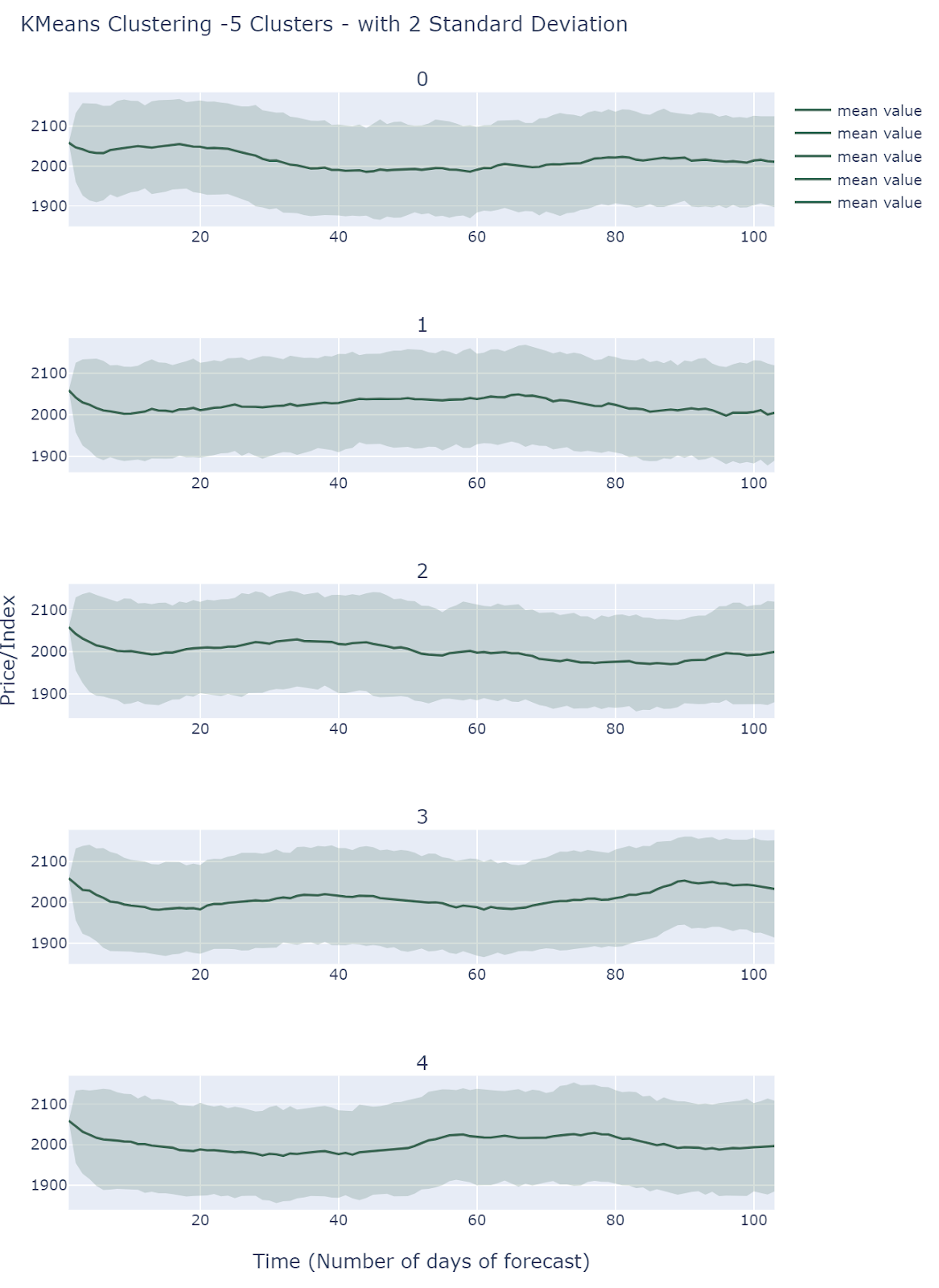
K-Means Clustering of Scenarios
By default , we choose 5 clusters using L2-K-Means clustering to extract different scenarios.
All Clusters behave differently and they all fall into comparable ranges. Simulations does show different scenarios but it is still unclear how to interpret these results.
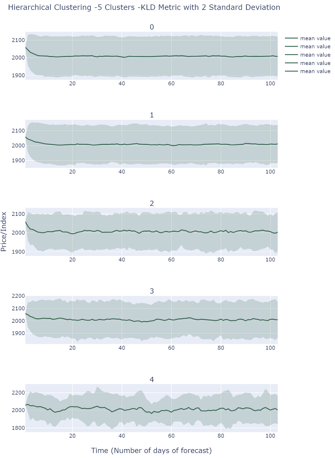
Hierarchical Clustering of scenarios
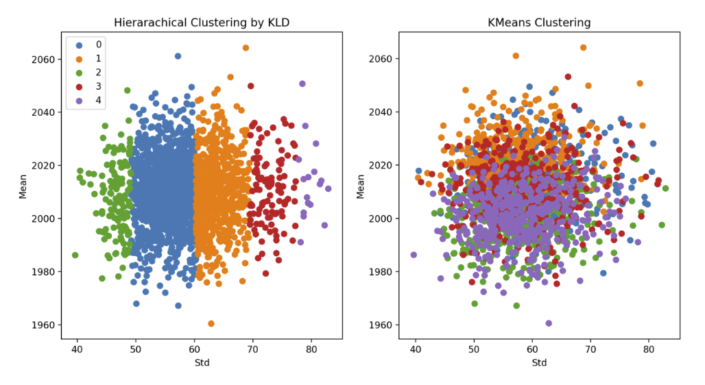
By default , we choose 5 clusters using Hierarchical Clustering(KL Divergence Affinity) to extract different scenarios. Cluster 0 and 1 presents relatively low volatilities, and cluster 2 and 3 shows medium volatilities. Cluster 4 is the most volatile one among all clusters. Therefore, Hierarchical Clustering method groups observations based on volatility.
 .
.
Clustering Comparison
Clustering is a method allowing us to focus on major patterns reflected by the simulation. KMeans seems only able to identify outliers, almost impossible situations but KLD Hierarchical Clustering is able to separate scenarios based on the volatility imply stable and a little less stable future is most likely to happen.
