Description of the problem

In this exercise, we will analyze the financial vital signs for bankruptcy. First, we will identify 66 failed firms from a list provided by Dun and Bradstreet. These firms were manufacturers or retailers, whose financial data was available on the Compustat Research tape. Bankruptcy occurred somewhere between 1970 and 1982. The dataset also contains information about "healthy firms".

The aim of this analysis is to see how well bankruptcy can be predicted two years in advance. The table below is 24 features that describe 132 firms based on the Compustat tapes and Moody's Industrial Manual for the year that was two years prior to the year of bankruptcy.

The first four features with CASH in the numerator can be considered as a firm's cash reservoir with which to pay debts. The three features with CURASS are the firm's generation of current assets with which to pay debts. Two features, CURDEBT/DEBT and ASSETS/DEBTS, measure the firm's debt structure. Inventory and receivables turnover are measured by COGS/INV and SALES/REC, and SALES/ASSETS is the firm's ability to generate sales. The rest of the 12 features are asset flow measures.

What you will build

• Random forest model

What you will learn

• Explore the dataset by using pandas, numpy, matplotlib.
• Compare the performance of Logistic Regression, Random Forest Classifier and Multi-layer Perceptron classifier.
• Select significant features for new model.
• Build Random Forest Classifier for classification.
• Use confusion_matrix, ROC curve and cross-validation to evaluate model performance.

• pandas
• numpy
• matplotlib
• sklearn
• xlrd
• seaborn

First, use pandas pd.read_excel to read the excel file. Since the dataset does not have any invalid value, you can skip the step of cleaning the data. To check invalid value, you can use df.isnull()

Have a look at top 5 rows in the dataset (part of the columns):

Split the dataset into df_D0 where D=0 (bankruptcy/failed firm) and df_D1 where D=1 (healthy firm) and plot the mean value of each features in 2 classes.

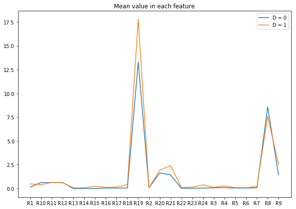
From the plot, we can see some difference in R19, R21 and R8 between healthy companies and failed firms, however, there is not much difference in other features.
Next, plot the time distribution of the bankruptcy over time, and then plot the distribution of each feature.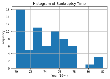

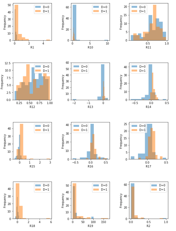
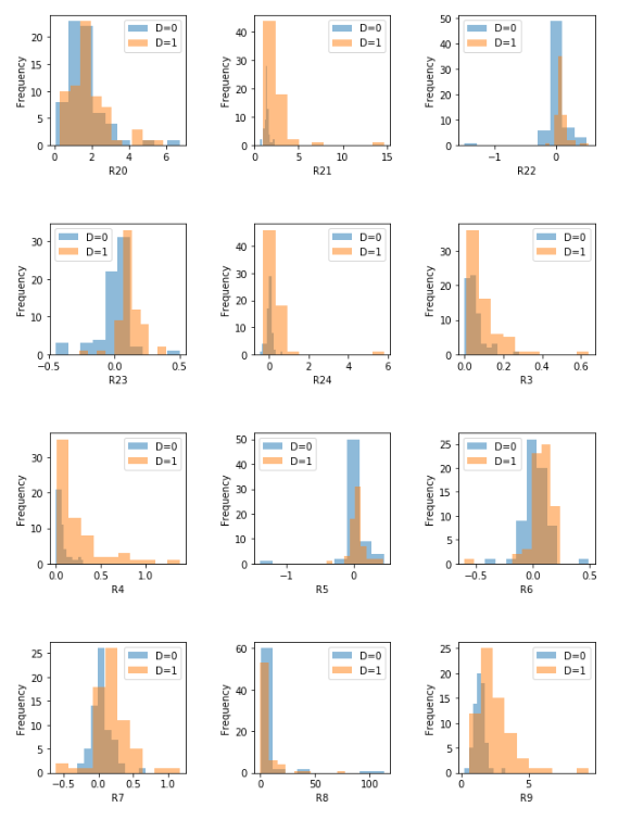
From the plots, you might be able to find that:

• Features whose distributions (D=0, D=1) have more significant difference, such as R17, R22, and R23, may be a better predictor of the bankruptcy.
• Features whose distributions (D=0, D=1) have less significant difference, such as R19, R12 and R5 may be a bad predictor of the bankruptcy.
  

Since each failed firm has an opposite healthy firm, in order to train a nice model, you can collect pairs of corresponding firms in the same train/test dataset.

Hyperparameter tuning for Logistic Regression, Random forest classifier and Multi-layer Perceptron classifier with 5-fold cross validation. Then, select the model with the best performance.

Result:

As the best performance report of each model shown below, we select the model that has the highest accuracy score: Random Forest Classifier. Accuracy score (the number of correct predictions / the total number of predictions) is important since our goal is to correctly predict bankruptcy.

Now, you can use the training set to build a random forest classifier model with the best parameters. Best parameters are:

Best max_depth: 3

Best max_features: 5

Best min_samples_split: 2

Best min_samples_leaf: 3

Best bootstrap: False

Best criterion: gini

Best random_state: 5

Best score: 0.8653846153846154

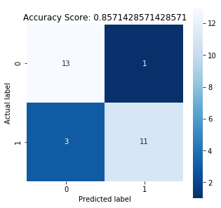
In the notebook, the accuracy is 0.8571428571428571

You can check the confusion matrix of the test set and plot a heatmap to visualize the confusion matrix.

Plot the ROC curve:

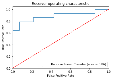
Then, print out the performance report for your model. The performance of the model in the notebook is:

To improve a model, you can select features that influence the model more. There are two ways to select the significant features in the notebook.

Selecting features based on the ranking

The sorted feature_importances_ of the model in the notebook is:

[(0.12713, 'R7'), (0.12525, 'R14'), (0.11428, 'R18'), (0.10584, 'R21'), (0.1009, 'R15'), (0.09672, 'R9'), (0.06942, 'R17'), (0.03759, 'R24'), (0.03565, 'R13'), (0.03287, 'R1'), (0.03123, 'R6'), (0.02182, 'R11'), (0.02084, 'R20'), (0.01721, 'R16'), (0.01696, 'R4'), (0.01606, 'R2'), (0.01, 'R12'), (0.0097, 'R23'), (0.00487, 'R5'), (0.00478, 'R10'), (0.00086, 'R8'), (0.0, 'R3'), (0.0, 'R22'), (0.0, 'R19')]

After selecting top 15 significant features for a new model, the accuracy becomes 0.893. Compared with the old model, the score improved. When selecting 10 or 30 significant features, however, the accuracy decreases.

Removing multicollinearity

Multicollinearity occurs when your model includes an independent variable that are highly correlated with multiple variables. It may increase the standard errors of the coefficients, which will make some variables statistically insignificant even when they should be significant. In order to select actual significant features, you may need to remove highly correlated predictors from the model.

In the notebook, we plot the heatmap to see the correlation between each features and then select the high correlation pairs manually.

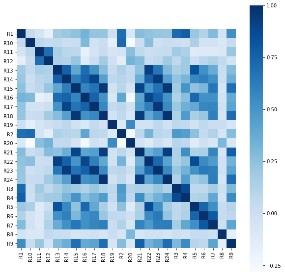
Then, considering the feature importance, we keep one of the features in each pair that is the most important and delete the others. The new heatmap of correlation is shown below:

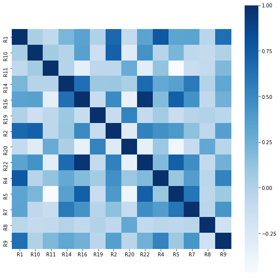
Even after removing highly correlated predictors from the model, the accuracy did not decrease. This indicates that our model might face the multicollinearity problem.

Build a model with one or two features

When using one feature for the model, the result should look like this:

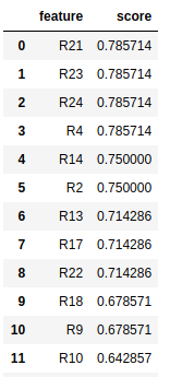
You can see the top 4 scores, R21, R23, R24 and R4 are the exact same. Now you can also try to use two features to train the model. When R4 and R23 are used, for example, the score increases a little to 0.8214, which shows that these two features are independent, giving more value to the model.

But when training the model with feature R4 and R21 (their single feature prediction scores are 0.7857), the score slightly decreases to 0.714, which means these two features may have high correlation, but they cannot give much value to the new model when combined.

Using box-plot

Now, we can explore the data to gain a deeper understanding of which variables may be important in distinguishing bankrupt from non-bankrupt firms by using box-plot for each feature.

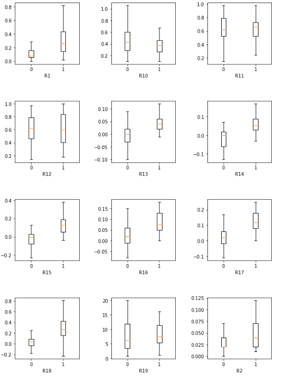
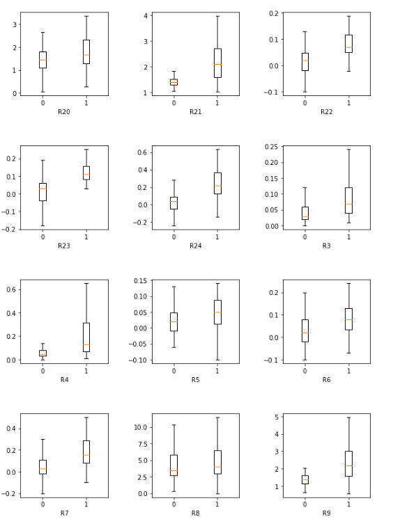
From the plots, you may find that:

• Important features: R1, R3, R9, R11, R13, R15, R16, R17, R18, R21, R23, R24.
• In the feature R1, R4, R9, R18 and R21 figures, there is almost a clear line between the range of bankruptcy and healthy company. Furthermore, the box plots of healthy firms are much higher than the failed ones. Also, the box plots of the failed firms have much smaller range, which indicates the value is very concentrated. This can be said those features are important in making decisions to decide whether a company will go bankrupt or not.

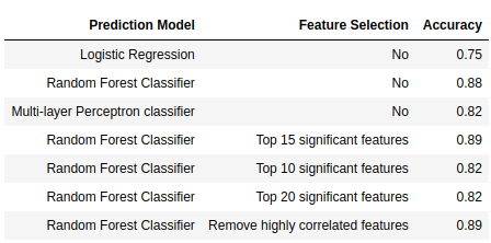
The table below is accuracy result for each prediction model with different feature selection. Random Forest Classifier with highly-correlated features removed and the one with 15 significant features have the highest accuracy score. Box-plot also provides an opportunity to understand which features to pay attention to when making a decision.

Shmueli.G, Bruce.P.C, Patel.N.R (2016) Data Mining For Business Analytics (Third Edition)