Description of the problem
The understanding of the appliances energy use in buildings has been the subject of numerous research studies, since appliances represent a significant portion (between 20 and 30%) of the electrical energy demand. For instance, in a study in the UK for domestic buildings, appliances, such as televisions and qne consumer electrical energy consumption in buildings can be useful for a number of application: to determine adequate sizing of photovoltaics and energy storage to diminish power flow into the grid, to detect abnormal energy use patterns, to be part of an energy management system for load control, to model predictive control applications where the loads are needed, for demand side management (DSM) and demand side response(DSR) and as an input for building performance simulation analysis.
What you will build
- Linear regression
- Random forest regressor
- Gradient boosting regressor
- Support vector machine regressor
What you will learn
- Perform exploratory data analysis (EDA) on data
- Apply feature engineering based on the data set and feature selection using RFE, Boruta and .feature_importance_ attribute of regressors in sklearn
- Use models in sklearn to build, train data, tune hyperparameter using grid search with cross validation and evaluate their performances using different error metrics
- pandas
pandas is an open source, BSD-licensed library providing high-performance, easy-to-use data structures and data analysis tools for the Python programming language
- scipy
SciPy (pronounced "Sigh Pie") is a Python-based ecosystem of open-source software for mathematics, science, and engineering
- numpy
NumPy is the fundamental package for scientific computing with Python. It contains among other things: a powerful N-dimensional array object; sophisticated (broadcasting) functions; tools for integrating C/C++ and Fortran code; useful linear algebra, Fourier transform, and random number capabilities
- matplotlib
Matplotlib is a Python 2D plotting library which produces publication quality figures in a variety of hardcopy formats and interactive environments across platforms. Matplotlib can be used in Python scripts, the Python and IPython shells, the Jupyter notebook, web application servers, and four graphical user interface toolkits
- seaborn
Seaborn is a Python data visualization library based on matplotlib. It provides a high-level interface for drawing attractive and informative statistical graphics
- sklearn
Sklearn is a free software machine learning library for the Python programming language. It features various classification, regression and clustering algorithms including support vector machines, random forests, gradient boosting, k-means and DBSCAN, and is designed to interoperate with the Python numerical and scientific libraries NumPy and SciPy
- boruta
Python implementations of the Boruta R package. This implementation tries to mimic the scikit-learn interface, so use fit, transform or fit_transform, to run the feature selection
Dataset Description and Visualization
Load the data
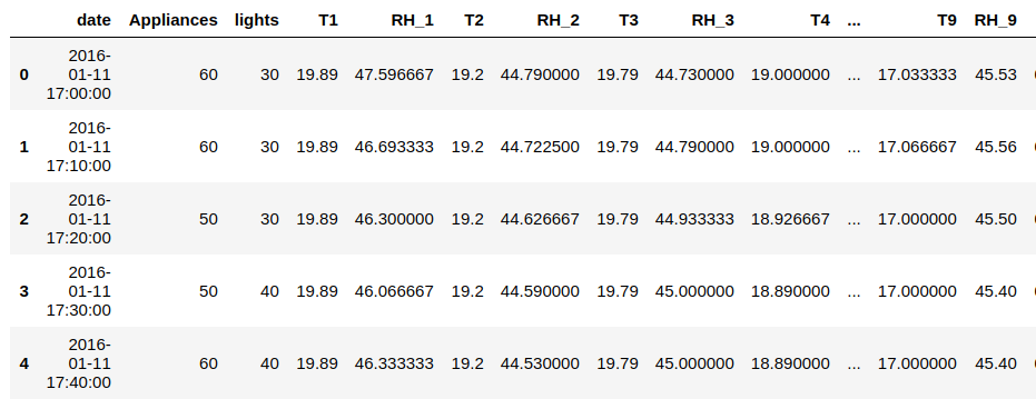
Use pd.read_csv(‘path_to_the_file') to load the data set (csv file) as a pandas dataframe. Call dataframe.info() to check the data type and missing value counts in the data set. Since there is no missing value or invalid value in the data set, we can skip the data cleaning step. By calling dataframe.head(), we can have a look at the first 5 rows of the data set to see what the data set looks like:
Also, we can use series.value_counts() on the categorical columns to see if there is any odd values need to be handled.
Energy Consumption Measurement on Date
Firstly, we might want to see the energy consumption distribution on the date using matplotlib. Before plotting, we need to convert the ‘date' values in the data set to standard datetime format by calling pd.to_datetime().

The energy consumption profile shows a high variability. Some kind of periodicities might be found but not very obvious. Let us have a closer look at the first week of data to see is there any pattern to be found.

As we can see in the above graph, there are two peaks in a day. The energy consumption is comparatively high in the morning and evening, which is easy to understand, when people might use more appliances after waking up or getting home from work. To verify this idea, we could use a heatmap which might give us a clear picture of the consumption differences based on hour of day.
Heat Map
A heat map is a two-dimensional representation of data in which values are represented by colors. A simple heat map provides an immediate visual summary of information. More elaborate heat maps allow the viewer to understand complex data sets. We will plot heat map using seaborn library.
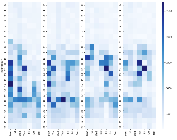
The heat map does show a strong pattern based on hour of day. The heat (which actually means the energy consumption) rises significantly in the morning around 8 and 9 and keeps a high level in the noon. From 18 to 19, there is another hot spot. After 20, the heat starts to fall.
The energy consumption measurement on date and the heat map on hour of day strongly indicate that the appliances energy consumption is related to time of day. The 'date' in our dataset is in a standard datetime form which is easy for us to understand but not good for computation and model fitting. Thus, a new feature need to be defined in our dataset to present the specific time of day based on 'date'. Also, it seems the heat in weekdays and weekends differ from each other. Even there might be some patterns based on day of week which we cannot tell. Thus, we might add these features in feature engineering to fully use the data set.
Let us convert 'date' to 'Number of Seconds from Midnight' using the following code:
df['NSM'] = pd.to_datetime(df.date)-pd.to_datetime(df.date.str.split('\s+').str[0]+" 00:00:00")
def time_to_second(time):
    return time.total_seconds()
df['NSM'] = df['NSM'].apply(time_to_second)
df.head()
Energy Consumption Distribution
- Histogram
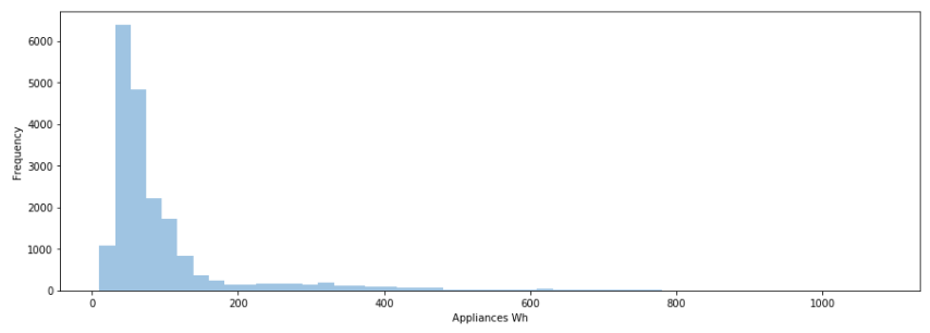
The histogram shows the frequency of energy consumption in different value intervals. As we can see, most of the observations are located between 20 and 100.
- Boxplot
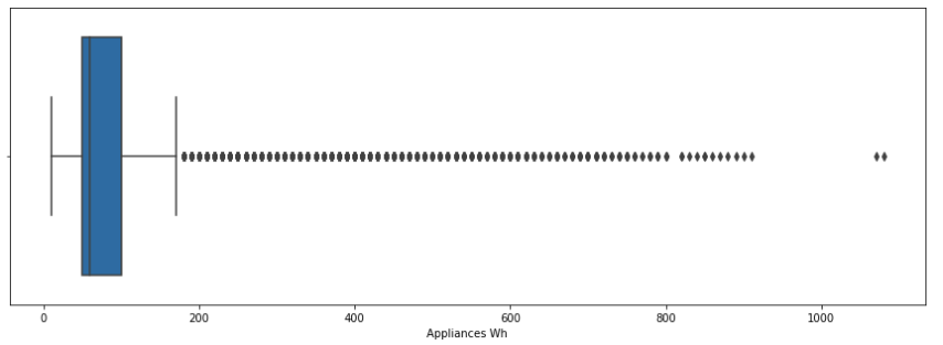
The long tail of the box plot indicates that there are some large values with very low frequencies. The box plot also shows the median value which is 60 Wh. The lower whisker of the box is 10 Wh and the upper whisker is 175 Wh.
Pairwise Analysis
Data set split
train, test = train_test_split(df, test_size=0.25, random_state=10)Use sklearn.model_selection.train_test_split() to split the data set into train set and test set. Let us consider the test set (which is 25% of our complete data) is unknown. We will only use the train set for the following analysis. Test set will only be used for prediction.
Pair plot
We can use seaborn.PairGrid() to generate pair plot. To show the pearson correlations parameters on the upper side above the diagonal, another function need to be defined to calculate the parameters using scipy.stats.pearsonr(). Then pass this function to the .map_upper attribute of the pair plot. The pearson parameters are clearly listed on the plot and a summary table is created to rank the parameters in descending order (please check the bottom of jupyter notebook).
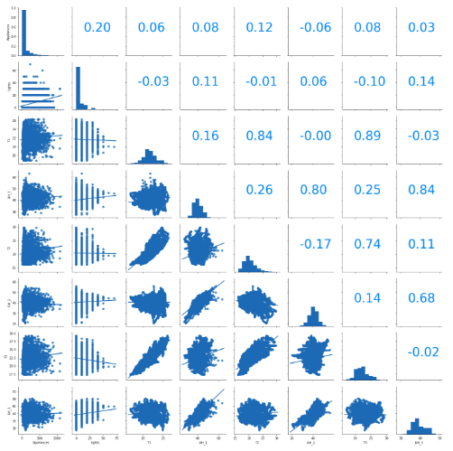
We can conclude that Number of seconds from midnight (NSM), light energy consumption (lights), temperature in living room area (T2), temperature outside the building (T6) and temperature outside the weather station (To) present stronger positive correlations with appliance energy consumption compared with other variables. This actually support our idea of adding 'NSM' into our data set according to the data visualization based on hour of day. The only two features that has a negative Pearson Correlation coefficient more negative than or equals to -0.10 are humidity outside the weather station (RHo) and humidity in teenager room2 (RH8).
There are actually some other features which have a very high correlation to each other. Temperature in ironing room (T7) and temperature in parents room (T9) have a coefficient of 0.94. You might heard it is bad to have highly related features in supervised learning. However, Correlated features will not always worsen your model. On the other hand, they will not always improve it either. You can remove highly correlated features if you are concerning the following factors:
- Make the learning algorithm faster
- Decrease harmful bias
- Interpretability of your model
These pair plots can just give us a overall picture of correlations between features. I would definitely recommend you to do feature selection if you really want to detect high correlated features and handle them for a better prediction.
Feature engineering is the process of using domain knowledge of the data to create features that make machine learning algorithms work. Feature engineering is an informal topic, but it is considered essential in applied machine learning.
In this part, feature engineering is applied to the dataset we described in the last part. Since the dataset has already been cleaned (no missing value or odd categorical value) and there are no text features, no image features in the dataset, the main task of feature engineering will be generating new feature (NSM) and dummy variables of categorical features.
Load the data
Use pd.read_csv(‘path_to_the_file') to load the data set (csv file) as a pandas dataframe.
Add 'Number of Seconds from Midnight'
According to data visualization and exploratory analysis, the specific day time does affect the appliance energy consumption. Thus, we need to convert 'date' into 'NSM' (number of seconds from midnight) here just like what we did before pairplot analysis.
Add 'Day of Week'
Day of week is added using dt.weekday_name. This function will return the name of the weekday according to the date time it gets from .to_datetime(df.date).
Add 'Weekday Status'
def weekday_status(day):
    if day == 'Saturday' or day == 'Sunday':
        return 'Weekend'
    else:
        return 'Weekday'
We can define a function like above to decide whether the day for week is in weekend or weekday. The function need to be passed as an argument to .apply() function of the ‘day of week' column.
Generate Dummy Features
The very first idea for transferring categorical data like ‘day of week' is simply assign the value of the day as a integer from 1 to 7. Similarly, assign the value of weekday status to binary value like 0 and 1. However, the regression models inside the python packages make the fundamental assumption that numerical features reflect algebraic quantities. For example, that Monday < Tuesday < Wednesday<..., or even that Sunday - Saturday = Monday, which does not make much sense.
Thus, one-hot encoding should be applied here, to generate dummy columns indicating the presence or absence of a category with a value of 1 or 0, respectively.
Then the ‘Day_of_week' and ‘Weekstatus' columns are transformed to dummy variables using pandas.get_dummies().
Let us have a look at what we just generated in the original data set:

Train / test split
Before we moving on to model fitting, we have to split the data set into train set and test set with a proportion of 3/1 using sklearn.model_selection.train_test_split(). Test set is assumed to be unknown and will only be used for testing the models' performances (Noticed that specify a value of random_state in the train_test_split() function will give you the same train / test set every time to ensure the consistency of the analysis). Also, we need to save the train / test set to a csv file for further use.
train.to_csv('datasets/training.csv', index=False)
test.to_csv('datasets/testing.csv', index=False)
In this part, we will try out Linear Regression, Random Forest, Gradient Boosting and Support Vector Machine to do regression on this data set. We will not do any further model selection here and will just use the default model in Sklearn to have a general sense of their performances.
After loading the train set and test set, we will generate the predictors (X) and targets (y). Except 'Appliances' and 'date', we also remove another 4 features in predictors:
- 'rv1', 'rv2' are two random variables which have no predicting power for the appliances' energy consumption.
- In many cases, if a categorical feature is transferred into N dummy features, only (N-1) dummy features will be used. We can always know the value of Nth dummy feature according to the other (N-1) values. Thus, we remove 'Day_of_week_Sunday' and 'WeekStatus_Weekend' here.
We will use DummyRegressor as our baseline model. By default, DummyRegressor will always predict the mean of the training set no matter which observation it is dealing with.
The performances of all the 5 (including benchmark) models are shown as follows:

As we can see from the table above, machine learning models have stronger predicting power than a baseline model except SVM. Again, we just used default models to get a general sense of their performances. And if a test set RMSE of 71.02 and test set MAPE of 33.42 is acceptable for you, you can stop right here and say that Random Forest is good enough to predict the appliances energy consumption in this case. Otherwise, you might want to find more fittable hyperparameter sets for these models to improve their performances and to see which one is the real optimal one.
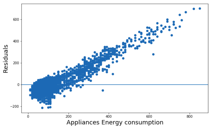
Also, above is a residual plot for the linear regression model. The residuals were computed as the difference between the real values and the predicted values. From the plot, it is obvious that the relationship between the variables and the energy consumption of appliances is not well represented by the linear model since the residuals are not normally distributed around the horizontal axis. We will not discuss linear regression further in this case.
In this part, we will be using three different methods to implement feature selection on all three models:
- Recursive Feature Elimination (RFE)
- Boruta
- Feature Importance
Feature Ranking Methods
Given an external estimator that assigns weights to features (e.g., the coefficients of a linear model), the goal of RFE is to select features by recursively considering smaller and smaller sets of features. First, the estimator is trained on the initial set of features and the importance of each feature is obtained either through a coef_ attribute or through a feature_importances_ attribute. Then, the least important features are pruned from current set of features. That procedure is recursively repeated on the pruned set until the desired number of features to select is eventually reached.
Recursive Feature Elimination (RFE) with Cross Validation
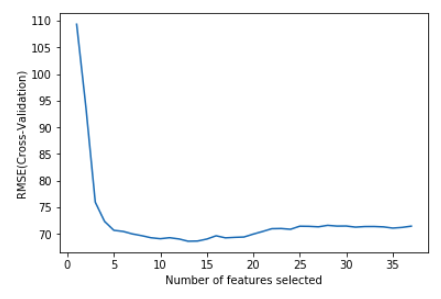
As we can see from the graph above, 13 will be the optimal number of features calculated by RFE using Random Forest model. We can use .support_ attribute to extract these 13 features.
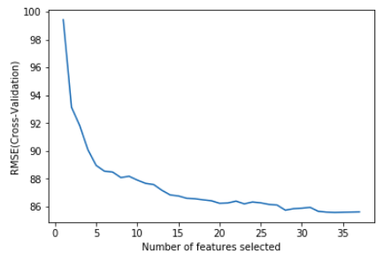
This is the results generated by RFE using GBM. 34 is the optimal number which means we will use almost all the features in the model selection including the two random variables which have nothing to do with improving the predicting result. Thus, we will not be testing the features selected by RFE with GBM.
Boruta
This is an all-relevant feature selection method. It tries to capture all the important, interesting features you might have in your dataset with respect to an outcome variable. You can check the complete implementation of Boruta using this url: http://danielhomola.com/2015/05/08/borutapy-an-all-relevant-feature-selection-method/
Using Boruta with Random Forest gives us the optimal number of 16.
The transform of the predictors and targets could be done by the following code:
X_train_boruta = X_train.values
y_train_boruta = y_train.values.ravel()
X_test_boruta = X_test.values
y_test_boruta = y_test.values.ravel()
Variable Importance (Sklearn)
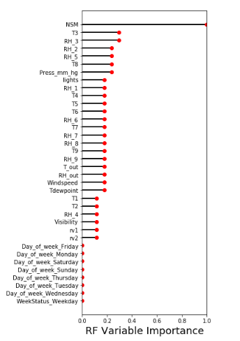
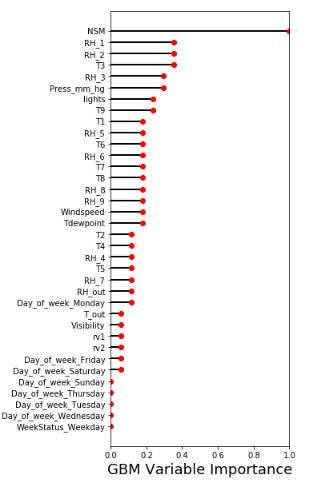
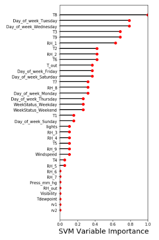
For ensemble models in Sklearn like Random Forest and Gradient Boosting, we can use .feature_importances_ attribute to get the importances of all the features for the specific model. For the SVM, the relationship between each predictor and the outcome is evaluated and then a linear model is fit and the absolute value of the t value for the slope of the predictor is used.
- Random Forest
As we can see from the graph below, .feature_importance_ can actually determine the two random variables as unimportant features. There are several gradients in the graph based on the importance score. We can consider different feature selection sets to test the prediction power according to the score. For example, we can simply test with the features with their importance greater than 0.01 or 0.02. Same thing for GBM and SVM.
- Gradient Boosting
- Support Vector Machine
Feature Selection
In this part, we will train/test the data using different sets of features to compare their performances. The performances are measured by RMSE calculated by 5-fold cross validation.
Here is the result of the feature selection:
- Random Forest

- Gradient Boosting

- Support Vector Machine

According to the metrics: Random Forest works best with 13 features selected by RFE algorithm. Gradient Boosting reaches the best performance using all the features. Support Vector Machine performs better with features having importances greater than 0.02.
The next thing we are going to do is generating different csv files of train/test set with different features for different models. So that we can easily load any specific data set we want to use for fitting specific model.
Tuning Hyperparameters
Random Forest Regressor
For Random Forest, hyperparameters that were tuned in our project are:
- n_estimators: the number of trees in the forest.
- max_depth: the maximum depth of the tree. If None, then nodes are expanded until all leaves are pure or until all leaves contain less than min_samples_split samples.
- max_features: the number of features to consider when looking for the best split.
Grid search with 3-fold cross validation (you can definitely use a larger number of folds to increase the precise of the result) was used in the hyperparameter tuning using the following code (Similar for GBM and SVM):
# Create the parameter grid
param_grid = {
    'max_depth': [30, 50, 70, 110],
    'max_features': [0.7, 0.8, 0.9, 'auto'],
    'n_estimators': [100, 200, 300, 500]
}
# Create a based model
rf = RandomForestRegressor()
# Instantiate the grid search model
grid_search = GridSearchCV(estimator = rf, param_grid = param_grid,
                          cv = 3, n_jobs = -1, verbose = 2)
The result showed that the optimal Random Forest model for this problem is the one with n_estimators = 300, max_depth = 160, max_features = 0.7.
Gradient Boosting Regressor
For GBM, hyperparameters that were tuned in our project are:
- n_estimators: the number of boosting stages to perform. Gradient boosting is fairly robust to over-fitting so a large number usually results in better performance.
- max_depth: maximum depth of the individual regression estimators. The maximum depth limits the number of nodes in the tree. Tune this parameter for best performance; the best value depends on the interaction of the input variables.
The result showed that the optimal Gradient Boosting Regressor model for this problem is the one with n_estimators = 5000, max_depth = 9.
Support Vector Regressor
For SVM, hyperparameters that were tuned in our project are:
- gamma: kernel coefficient for ‘rbf', ‘poly' and ‘sigmoid'. If gamma is ‘auto' then 1/n_features will be used instead.
- C: penalty parameter C of the error term.
The result showed that the optimal Support Vector Regressor model for this problem is the one with gamma = 0.1, C = 900.
Conclusion

The table above shows the performances of all models before and after tuning hyperparameters. As we can see, all models perform better after tuning especially for Support Vector Regressor.
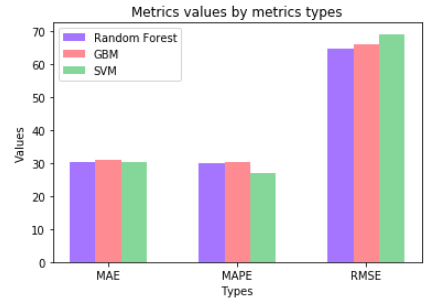
Here is the performance of all the optimal models after tuning hyperparameters:

Before we come to the conclusion, let me first explain these three metrics detailedly:
MAE refers to Mean Absolute Error. It gives less weight to outliers, which is not sensitive to outliers. MAPE refers to Mean Absolute Percentage Error, which is similar to MAE, but normalized by true observation. Downside is when true obs is zero, this metric will be problematic.
MSE refers to Mean Squared Error, which is like a combination measurement of bias and variance of your prediction, i.e., MSE = Bias^2 + Variance, which is also most popular one I guess. RMSE refers to Root MSE, usually take a root of MSE would bring the unit back to actual unit, easy to interpret your model accuracy. Taking the square root of the average squared errors has some interesting implications for RMSE. Since the errors are squared before they are averaged, the RMSE gives a relatively high weight to large errors. This means the RMSE should be more useful when large errors are particularly undesirable.
RMSE has the benefit of penalizing large errors more so can be more appropriate in some cases, for example, if being off by 10 is more than twice as bad as being off by 5. But if being off by 10 is just twice as bad as being off by 5, then MAE is more appropriate.
From an interpretation standpoint, MAE is clearly the winner. RMSE does not describe average error alone and has other implications that are more difficult to tease out and understand.
On the other hand, one distinct advantage of RMSE over MAE is that RMSE avoids the use of taking the absolute value, which is undesirable in many mathematical calculations (not discussed in this article, another time...).
The above bar chart shows that the three models have very similar performances according to MAE, MAPE and RMSE. Generally, Random Forest with the selected features and hyperparameters is the best among the three. SVM has the smallest MAPE and the biggest RMSE. If we consider the total error generated by the model, then SVM is the worst one. However, if we care more about the difference between individual observation's predicting value and true value, then SVM is better than the other two.
I would say that the SVM can better describe the pattern behind the data and better catch the general relationships between energy consumption and other factors. However, if predicting the total energy consumption is the first priority, then Random Forest will be recommended.