This exercise will help one to learn how to build ARIMA/SARIMA models for time series data forecasting. Autoregressive integrated moving average(ARIMA) model is a generalization of an autoregressive moving average (ARMA) model. Both of these models are fitted to time series data either to better understand the data or to predict future points in the series. LSTM is a deep learning model which is popular in analyzing time series model. This exercise uses the Python packages to explore and analyze the swap rate data.
What you will build
You will first learn to visualize the time series data and decompose it into trend, seasonality and noise. Next, you will build ARIMA models and SARIMA models under different assumption and evaluate their forecasting performance. In the end you will also build a LSTM model to compare it with the previous linear models (namely ARIMA and SARIMA models). The exercise is established in Python 3.5.
What you will learn
Your learning objectives are:
- You will learn to do basic exploratory data analysis for time series data.
- You will learn how to build ARIMA/SARIMA model for forecasting.
- You will learn how to build LSTM model for time series analysis.
- You will learn to tune and evaluate the orders(hyperparameters) of the predictive models.
What you will need
You will need to:
- If you are doing the experiment on your own machine, you should first install Python 3.5, Jupyter notebook and the necessary packages list in the first cell of the notebook on your local machine. The instructions are listed in next part.
- You need to understand the basic concepts for time series analysis and machine learning. Don't worry if you are new in this area. Check the resource link below in ‘Prerequisite Knowledge' part.
What packages you need to install
Make sure you have installed Python 3.5, Jupyter notebook and the following packages. If you need any guide, check the links below:
- Python installation: https://www.python.org/downloads/release/python-366/
- Jupyter notebook installation: http://jupyter.readthedocs.io/en/latest/install.html
- Package installation example: https://pandas.pydata.org/pandas-docs/stable/install.html
- Necessary packages: pandas, numpy, matplotlib, datetime, statsmodels, sklearn
Where you can find the solution
You can find sample code in the solution for this exercise is included in swap_rates_forecast.ipynb.
Decomposition of time series data
To analysis time series data, a basic technology is to decompose it into different components, including trend, seasonality, noise(residual). One can see the long-run trend and seasonality more clearly in the decomposition process.
Check https://en.wikipedia.org/wiki/Decomposition_of_time_series for more information.
Stationary time series
Stationarity is a required assumption for ARIMA models. Hence before we build ARIMA models, we must make sure we can transform the original time series data into stationary time series data by de-trending and differencing.
Check the link below for the definition of stationarity and de-trending/differencing methods.
https://people.duke.edu/~rnau/411diff.htm
Cross-validation for time series data
Cross-validation process for time series data is a bit different from the normal data sets, because we can't select the data points randomly otherwise we will break the date/time order.
In order to use continuous training and validation data, we should use the similar strategy as follow:
- fold 1 : training [1], validation [2]
- fold 2 : training [1 2], validation [3]
- fold 3 : training [1 2 3], validation [4]
- fold 4 : training [1 2 3 4], validation [5]
- fold 5 : training [1 2 3 4 5], validation [6]
Description of the problem
In this case study, we will use the monthly swap rates data set obtained from www.Economagic.com. In the following questions, we are only interested in 1-year and 5-year maturities from July 2000 to May 2007. We will establish ARIMA/SARIMA models and LSTM model to perform short-term forecast of our target time series data.
After loading the necessary packages and the data. We can start to explore the swap rate data set.
Here are the first few lines of the original data set:

Decomposition of time series data
Since our first target is to fit ARIMA model to forecast 1-year swap rate, let's decompose the 1-year swap rate into different components as follows.
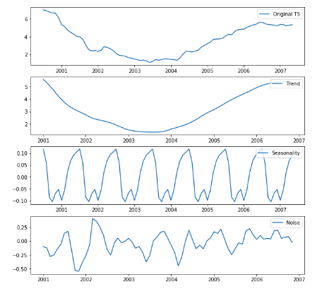
The time series decomposition shows:
- The trend decreased from 2000 to 2003, and after that 2004 it increased gradually until 2006.
- The time series has an annually seasonality.
- The noise(residual) seems random.
ARIMA model is a linear combination of AR(Autoregressive) model and MA(Moving Average) model. Check this link for more information about ARIMA model.
https://en.wikipedia.org/wiki/Autoregressive_integrated_moving_average
We use the ACF and PACF plots to determine the order of ARIMA/SARIMA models.
Let's first check the stationarity of the original data using Dickey-Fuller test.
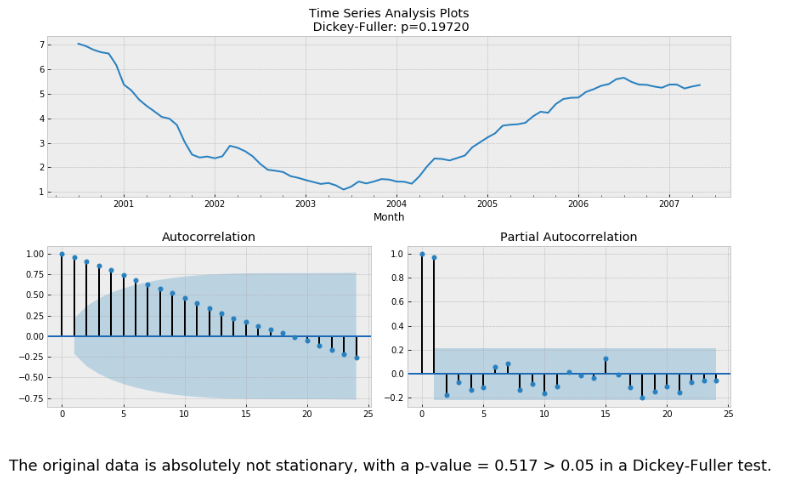
So we need to use detrending/differencing methods for stationarity transformation. Here we will use differencing for simplicity.
Differencing
If one use differencing to remove trend, then he/she need to use ARIMA model with constant trend component and d = the order of difference.
Let's take first difference and check stationary using Dickey-Fuller test.
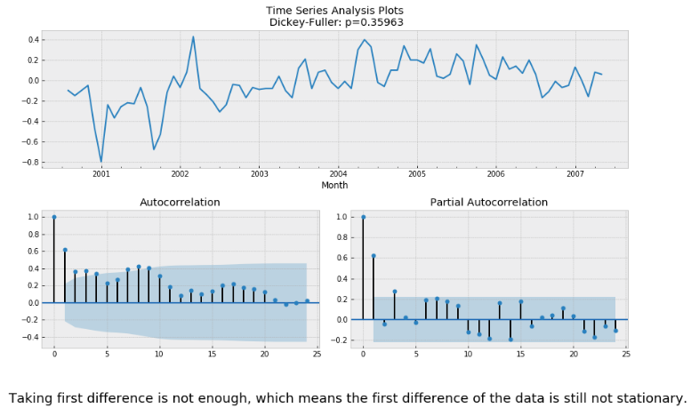
Taking first difference is not enough, which means the first difference of the data is still not stationary. Then we try to take the second difference of the data.
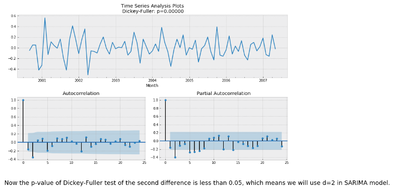
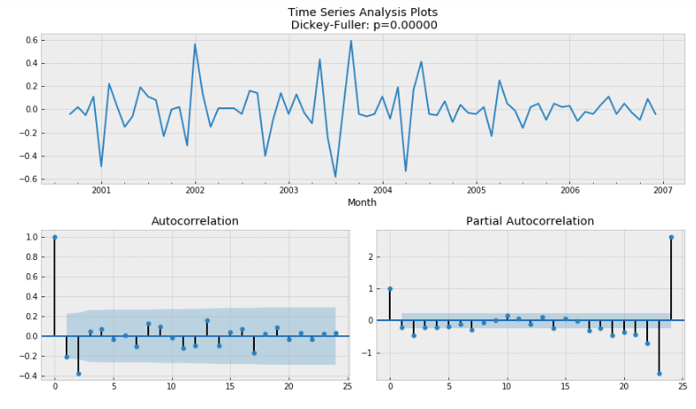
Now the p-value of Dickey-Fuller test of the second difference is less than 0.05, which means we will use d=2 in SARIMA model. Furthermore, from the ACFs and PACFs we know:
- p > 1, q > 1 because the ACFs and PACFs are not decrease exponentially.
- It's hard to say if P = 0 or 1, because the 12-th lag of PACF is on the bound of being significant.
- Q = 0, because 12-th lag of ACF is not significant
- D = 0, since we did take seasonal difference
- S = 12, since we have an annually seasonality for a monthly data.
Hyperparameter tuning for SARIMA model using cross-validation
To select the best orders for SARIMA model, we will do a cross-validation across different order combinations based on cross-validation MAPE score. By using the model selection function we defined in cell 21-22 in our sample code. We found the best model as follow:

Fit SARIMA model with tuned hyperparameters
We have find the best SARIMA orders based on our cross-validation process:
- seasonal_order = (0, 0, 0, 12)
- order = (2, 2, 1)
In-sample performance
Now let's first use all of our data as training data to see how well the model fits our data. The in-sample fitness result of this SARIMA model is shown as below.
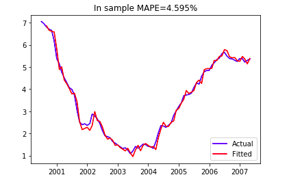
As one can see, the SARIMA model fitted in-sample data well with a 5% MAPE.
Out-of-sample performance
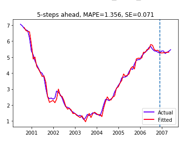
Here we use all the data before 2007 as our training data and compare our forecast with the actual swap rate in 2007. One can check the k-step ahead forecast in our sample code. Here we can see for 5-steps ahead forecast, we have out-of-sample MAPE as 1.356% which means we have a pretty close forecast value to actual values.
Now we want to build a SARIMA model to forecast the spread data, which is the difference between 1-year swap rate and 5-year swap rate. Below is the spread data from 2000 to 2007.

Check stationarity and differencing
In this part, one could check cell 35-37 in our sample code for the whole process of differencing. In this case the second difference is necessary for stationarity. Below is the Dickey-Fuller test and ACF/PACF plots for the second difference of the spread data.
Hyperparameter tuning
Now we compare the cross-validation MAPE on our validation sets and select the best orders for SARIMA model. Here we use our model selection function defined above again and get:

Hence the best model has order=(1,2,1) and seasonal_order=(0,0,0,12)). Next, let's fit the model with our training(insample) data. However, one will notice that even though our cross-validation shows the averaged MAPE is less than 10%, the forecast in test data is not good.
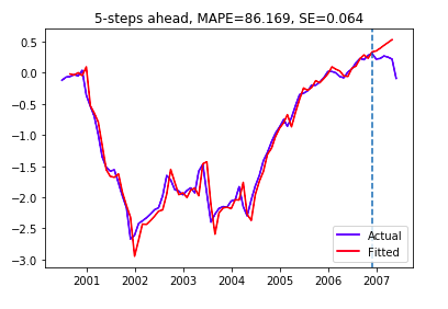
As one can see here, our SARIMA model can not predict the turning point of the spreads, its forecast keeps increasing. Comparing to the previous model, our model prediction is good for short-term prediction, because there is no turning points in our 5-steps ahead forecasts.
From the three exercises above, we observed that:
1. SARIMA fits data much better when there is seasonality in the target time series data.
2. In this case study, SARIMA model performs well for short term forecasting when there is not turning points in the forecast interval.
3. SARIMA model is not able to predict the turning points in future.
LSTM units are cells in a LSTM RNN(Recurrent Neural Network model) that can remember information over arbitrary time intervals. They have internal gates that help the cells 'input', 'forget' and 'output' information. The cells follow a recurrent pattern where data goes through a same cell over time. In the below figure, t represents the time.

Preparing Data for LSTM
LSTM models try to find a pattern from the sequence [0, 1, 2, 3, 4, 5] to → 6, while vanilla RNN models only focus on a pattern from [4] to → 6.
So if the input of a RNN model is:
- X : [0, 1, 2, 3, 4 ... 100]
The input for an LSTM would be some thing like:
- X : [[0, 1, 2, 3], [1, 2, 3, 4], [2, 3, 4, 5], .. [96, 97, 98, 99]]
LSTM Model
Some of the model hyperparameters include sequence length on one input sample, batch size, number of epochs, activation function, loss function and optimizer.
The model architecture can also be considered as a part of the hyperparameters. In this example we'll use a model with one LSTM layer with 8 neurons, followed by 2 dense layers having 2 and 1 neurons each respectively.
model = Sequential()
model.add(LSTM(8,input_shape=(seq_length,1),return_sequences=False))
model.add(Dense(2,kernel_initializer='normal',activation='linear'))
model.add(Dense(1,kernel_initializer='normal',activation='linear'))
model.compile(loss='mse',optimizer ='adam',metrics=['accur
acy'])
Prediction
Training Data: MAPE: 0.102%
Testing Data: MAPE: 0.107%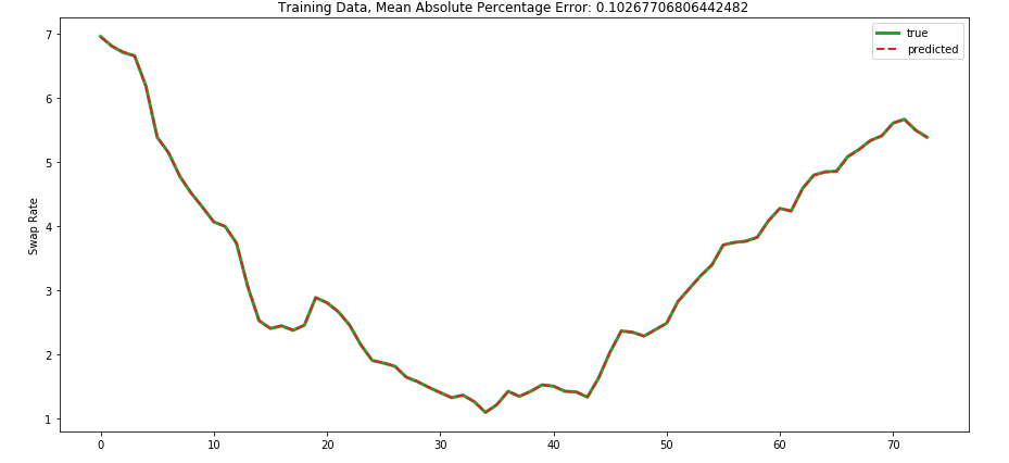
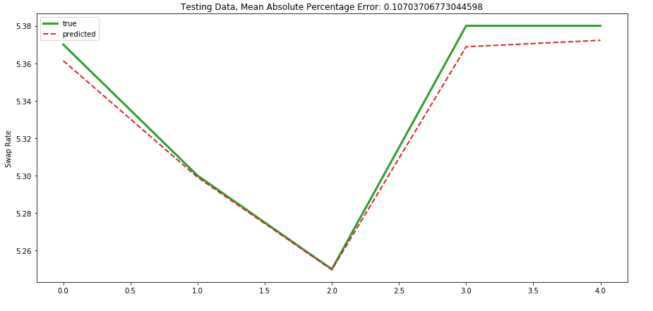
LSTM models fall under the deep learning category and usually require large amounts of data to have a better fit. Even though the results on the small data set are better than ARIMA models, we cannot ensure that this will perform better in all scenarios. This particular sample can also be considered as overfitting as the test sample size is very small to gauge its performance on wild data.