This exercise will help one to learn how to build ARIMA/SARIMA models for time series data forecasting. Autoregressive integrated moving average(ARIMA) model is a generalization of an autoregressive moving average (ARMA) model. Both of these models are fitted to time series data either to better understand the data or to predict future points in the series. ARIMA models are applied in some cases where data show evidence of non-stationarity, where an initial differencing step (corresponding to the "integrated" part of the model) can be applied one or more times to eliminate the non-stationarity.

This exercise uses the Python packages to explore and analyze the temperature anomalies data, and set up the predictive models to do long-term forecasts.

What you will build

You will first learn to visualize the time series data and decompose it into trend, seasonality and noise. Next, you will build ARIMA models and SARIMA models under different assumption and evaluate their forecasting performance. The exercise is implemented in Python 3.5.

What you will learn

Your learning objectives are:

1. You will learn to do basic exploratory data analysis for time series data.
2. You will learn how to build ARIMA/SARIMA model for forecasting.
3. You will learn to tune and evaluate the orders(hyperparameters) of the predictive models.

What you will need

You will need to:

1. If you are doing the experiment on your own machine, you should first install Python 3.5, Jupyter notebook and the necessary packages list in the first cell of the notebook on your local machine. QuSandbox has all the packages and installs in the experiment
2. You need to understand the basic concepts for time series analysis and machine learning. Don't worry if you are new in this area. Check the resource link below in ‘Prerequisite Knowledge' part.

What packages you need to install

Make sure you have installed Python 3.5, Jupyter notebook and the following packages. If you need any guide, check the links below:

1. Python installation: https://www.python.org/downloads/release/python-366/
2. Jupyter notebook installation: http://jupyter.readthedocs.io/en/latest/install.html
3. Package installation example: https://pandas.pydata.org/pandas-docs/stable/install.html
4. Necessary packages: pandas, numpy, matplotlib, datetime, statsmodels, sklearn

Where you can find the solution

You can find sample code in the solution for this exercise is included in temperature_analysis.ipynb.

Decomposition of time series data

To analysis time series data, a basic technology is to decompose it into different components, including trend, seasonality, noise(residual). One can see the long-run trend and seasonality more clearly in the decomposition process.

Check https://en.wikipedia.org/wiki/Decomposition_of_time_series for more information.

Stationary time series

Stationarity is a required assumption for ARIMA models. Hence before we build ARIMA models, we must make sure we can transform the original time series data into stationary time series data by de-trending and differencing.

Check the link below for the definition of stationarity and de-trending/differencing methods.

https://people.duke.edu/~rnau/411diff.htm

Cross-validation for time series data

Cross-validation process for time series data is a bit different from the normal data sets, because we can't select the data points randomly otherwise we will break the date/time order.

In order to use continuous training and validation data, we should use the similar strategy as follow:

• fold 1 : training [1], validation [2]
• fold 2 : training [1 2], validation [3]
• fold 3 : training [1 2 3], validation [4]
• fold 4 : training [1 2 3 4], validation [5]
• fold 5 : training [1 2 3 4 5], validation [6]

Description of the problem

In this problem, we are dealing with the temperature anomalies data from 1880-01 to 2010-08.

This is a monthly time series data. Our aim is to build ARIMA/SARIMA model to fit the in-sample data and do out-of-sample forecast. In this exercise one will see the limitation of linear models in long-term prediction. One could try modify the sample code to do short term prediction.

After loading the necessary packages and the data. We can start to explore the temperature anomalies data set.

Original time series data

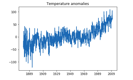
First, we can plot the original time series data. As one can see the temperature anomalies is oscillating around 0 before 1980, and after 1980, the temperature anomalies increases with a positive slope significantly.

Use moving average to observe the long-run trend

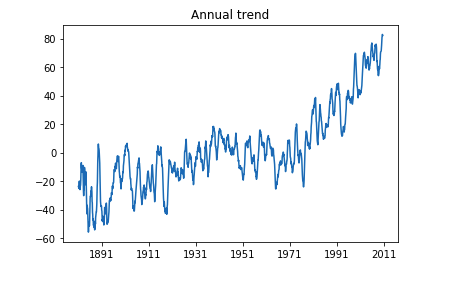
Since we have the monthly data as our original data, let's try smooth it using annual moving average methods. Namely, plot each point using the average of the 12 nearest data points instead of the actual value.

Use moving average in every decade

The previous one is not smooth enough, let's use a larger moving average window, say using the average in one decade.

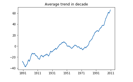
In this plot below you can see a much more clear trend of the data. Actually, before 1980, there was still a gradually increasing trend. After 1980 the slope become much steeper.

Decomposition of time series data

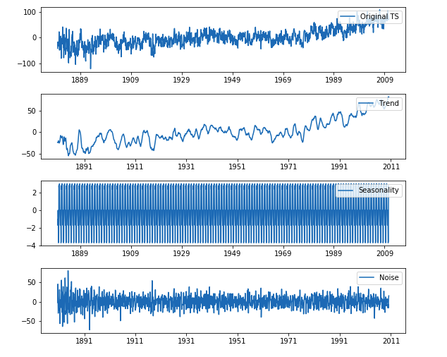
Now we can also decompose the data into different components: trend, seasonality, and noise.

From below, we can notice a gradually increasing trend and a annual seasonality.

ARIMA model is a linear combination of AR(Autoregressive) model and MA(Moving Average) model. Check this link for more information about ARIMA model.

https://en.wikipedia.org/wiki/Autoregressive_integrated_moving_average

We use the ACF and PACF plots to determine the order of ARIMA/SARIMA models.

Detrending and differencing for stationarity

AR model and MA model requires the time series to be stationary. Hence we need to use detrending or differencing to transform the raw data into a stationary data.

Let's first check the stationarity of the original data using Dickey-Fuller test.

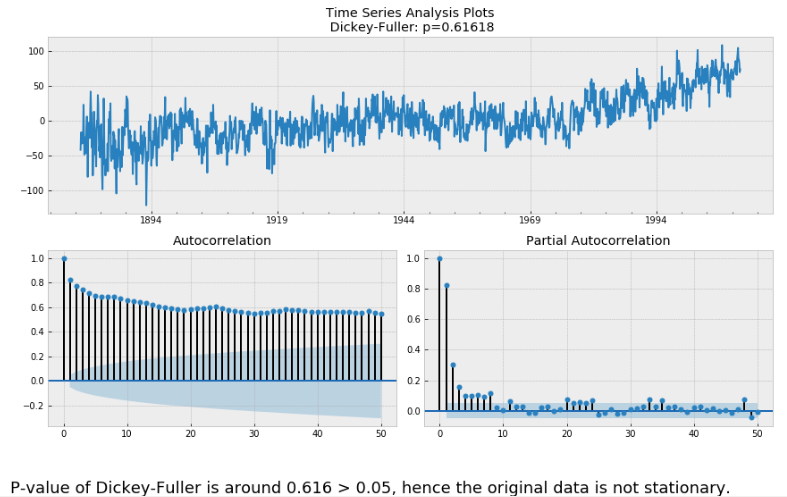
So we need to use detrending/differencing methods for stationarity transformation.

Differencing:

If one use differencing to remove trend, then he/she need to use ARIMA model with constant trend component and d = the order of difference.

Let's take first difference and check stationary using Dickey-Fuller test.

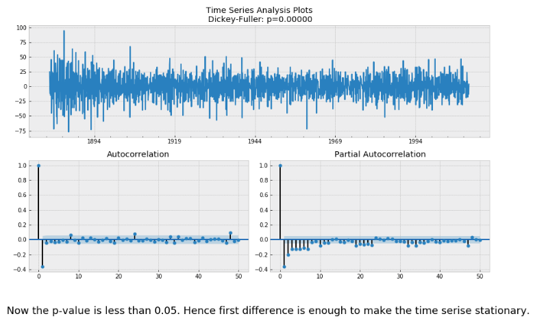
We can also determine the orders for ARIMA/SARIMA model based on the ACF/PACF plots.

• the ACFs are not significant after lag 2 except for lag 8, lag 24 and lag 48. Lags 8, 24, 48 are not as significant as the first two lags.
• the PACFs do not decay exponentially and the lag 1 is much larger than the following lags.

Hence, for simplicity we decide to set p = 1 , q = 2 and d = 1 (because we only take first difference to get stationarity) for our ARIMA model.

Detrending:

If one use detrend the data using linear model, then we need to build ARIMA model with linear trend component meaning that the original data it can be transformed into a stationary series by removing the effect of a time trend

Let's build a linear regression model with y= temperature anomalies, x=time, and check the stationarity of the residual.

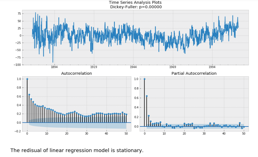
From the ACF and PACF plots:

• the residual is stationary, hence d = 0;
• the ACFs are all significant in finite lags, hence set q = 1, Q = 1 for simplicity;
• the PACFs do not decay in a exponentially, hence p > 1. So we use p = 2 for simplicity;
• the 12-th lag in PACFs is not significant, hence P = 0;
• We did not take seasonal difference to get a stationary data, hence D = 0;
• Here we consider annually seasonality for a monthly data, hence S = 12.

ARIMA model with constant trend:

(This model use differencing for stationarity transformation.)

Use all data as training data to fit the model and do a long time forecast:

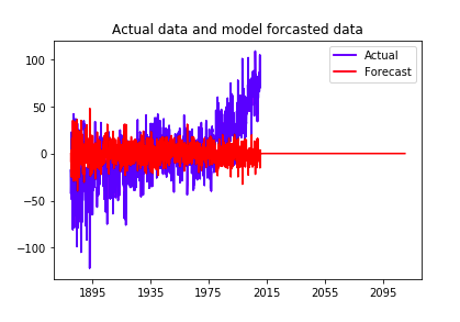
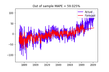
Evaluate out-of-sample forecast performance using last 200 points as test data:

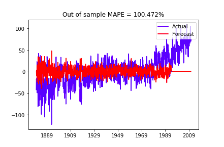
As shown above, the ARIMA model does not perform well both in-sample or out-of sample.

SARIMA model with constant trend:

(This model use differencing for stationarity transformation.)

Use all data as training data to fit the model and do a long time forecast:

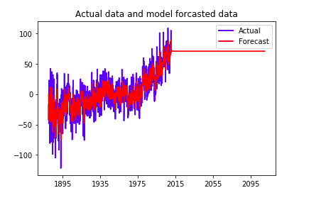
Evaluate out-of-sample forecast performance using last 200 points as test data:

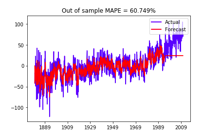
When we take seasonality into account and use SARIMA, we have a better in-sample fitness.

SARIMA model with non-constant trend:

(This model use detrending for stationarity transformation.)

Use all data as training data to fit the model and do a long time forecast:

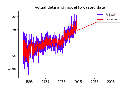
Evaluate out-of-sample forecast performance using last 200 points as test data:

Trend-shift model:

(This model use detrending for stationarity transformation.)

Use all data as training data to fit the model and do a long time forecast:

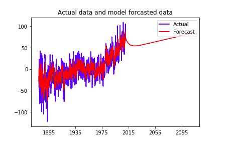
Evaluate out-of-sample forecast performance using last 200 points as test data:

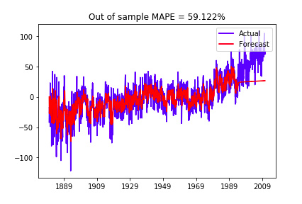
In this notebook, we have built ARIMA models and SARIMA models with non-constant/constant trends under different stationary assumptions. One can see that:

1. SARIMA model fits the data better when there is seasonality in the time series data.
2. The linear models(ARIMA/SARIMA) have limitation in long term prediction.
3. In this case study, the long term predictions we have in this notebook does not provide much useful information. However ARIMA/SARIMA models are good in short term predictions with small data set.