Summary
The goal of the p-median problem is to locating p facilities to minimize the demand weighted average distance between demand nodes and the nearest of the selected facilities. Hakimi (1964, 1965) first considered this problem for the design of network switch centers. However, this problem has been used to model a wide range of applications, such as warehouse location, depot location, school districting and sensor placement.
Problem Statement
The p-median problem can be formulated mathematically as an integer programming problem using the following model.
Sets | Set data that is used to define a model instance.
|
Parameters (Param) | Parameter data that is used to define a model instance.
|
Variables (Var) | Decision variables in a model.
|
Objective | Expressions that are minimized or maximized in a model.
|
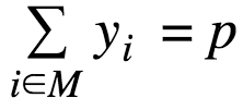
Constraints | Constraint expressions that impose restrictions on variable values in a model.
|
- pyomo
First, you need to declare an abstract model by creating a model object. The AbstractModel class provides a context for defining and initializing abstract optimization models in Pyomo when the data values will be supplied at the time a solution is to be obtained.
model = AbstractModel()Then, use Param function to declare the parameters m and n and use RangeSet component to declare the sets M and N abstractly.
# Number of candidate locations
model.m = Param(within=PositiveIntegers)
# Number of customers
model.n = Param(within=PositiveIntegers)
# Set of candidate locations
model.M = RangeSet(1, model.m)
# Set of customer nodes
model.N = RangeSet(1, model.n)
Similarly, the model parameters are defined abstractly using the Param component. The within option is used in these parameter declarations to define expected properties of the parameters. This information is used to perform error checks on the data that is used to initialize the parameter components.
For example, declare the "Number of facilities" parameter:
model.p = Param(within=RangeSet(1, model.n))Use the Var component to define the decision variables, which in this case is the flow over each arc. The within option is used to restrict the domain of the decision variables to the non-negative reals. This eliminates the need for explicit bound constraints for variables.
# x[i,j]-fraction of the demand of customer j tha tis supplied by facility i
model.x = Var(model.M, model.N,bounds=(0.0, 1.0))
# y[i]-a binary value that is 1 is a facility is located at location i
model.y = Var(model.M, within=Binary)
The Objective component is used to define the cost objective. This component uses a rule function to construct the objective expression
# Minimize the demand-weighted total cost
def cost_(model):
    return sum(model.d[j]*model.c[i,j]*model.x[i,j] for i in model.M for j in model.N)
model.cost = Objective(rule=cost_)
Similarly, rule functions are used to define constraint expressions in the Constraint component.
Finally, put these declarations all together and you will get your Pyomo model.
Since this is an abstract Pyomo model, the set and parameter values need to be provided to initialize the model. You can have a look at this synthetic data set:

This model is parameterized by three values: the number of facility locations, the number of customers, and the number of facilities.
Pyomo includes a pyomo command that automates the construction and optimization of models. The GLPK solver can be used in this simple example:
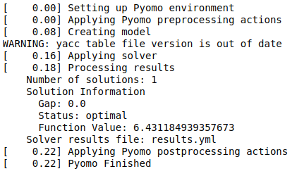
!pyomo solve --solver=glpk p-median.py p-median.datThis yields the following output on the screen:

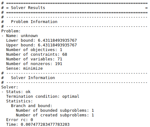
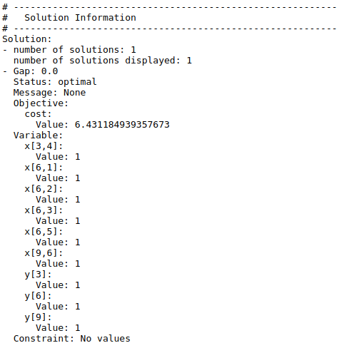
The numbers in square brackets indicate how much time was required for each step. Results are written to the file named results.yml, which as a special structure that makes it useful for post-processing.


This solution places facilities at location 3, 6 and 9. Facility 3 meets the demand of customer 4, facility 6 meets the demand of customers 1, 2, 3 and 5, and facility 9 meets the demand of customer 6.
- S.L. Hakimi (1964) Optimum location of switching centers and the absolute centers and medians of a graph. Oper Res 12:450–459
- S.L. Hakimi (1965) Optimum distribution of switching centers in a communication network and some related graph theoretic problems. Oper Res 13:462–475


