Summary

The goal of the Transport Problem is to select the quantities of an homogeneous good that has several production plants and several punctiform market as to minimise the transportation costs.

It is the default tutorial for the GAMS language, and GAMS equivalent code is inserted as single-dash comments. The original GAMS code needs slightly different ordering of the commands and it's available at https://www.gams.com/mccarl/trnsport.gms

Problem Statement

The Transport Problem can be formulated mathematically as a linear programming problem using the following model

• pyomo

Creation of the Model

In pyomo, everything is an object. The various components of the model (sets, parameters, variables, constraints, objective..) are all attributes of the main model object while being objects themselves.

There are two types of models in pyomo: A ConcreteModel is one where all the data is defined at the model creation. We are going to use this type of model in this tutorial. Pyomo however also supports an AbstractModel, where the model structure is firstly generated and then particular instances of the model are generated with a particular set of data.

The first thing to do in the script is to create a new ConcreteModel object. We have little imagination here, and we call our model "model". You can give another name, you also need to create a model object at the end of your script.

model = ConcreteModel()

Set Definitions

Sets are created as attributes object of the main model objects and all the information is given as parameter in the constructor function.

Specifically, we are passing to the constructor the initial elements of the set and a documentation string to keep track on what our set represents.

model.i = Set(initialize=[‘seattle', ‘san-diego'], doc='Canning plants')
model.j = Set(initialize=[‘new-york', ‘chicago', ‘topeka'], doc='Markets')

Parameters

Parameter objects are created specifying the sets over which they are defined and are initialised with either a python dictionary or a scalar:

For example:

model.a = Param(model.i, initialize={‘seattle':350, ‘san-diego':600}, doc='Capacity of plant i in cases')
model.b = Param(model.j, initialize={‘new-york':325, ‘chicago':300, ‘topeka':275}, doc='Demand at market j in cases')

A third, powerful way to initialize a parameter is using a user-defined function.

This function will be automatically called by pyomo with any possible (i, j) set. In this case, pyomo will actually call c_init() six times in order to initialize the model.c parameter.

def c_init(model, i, j):
    return model.f * model.d[i,j] / 1000
model.c = Param(model.i, model.j, initialize=c_init, doc='Transport cost in thousands of dollar per case')

Variables

Similar to parameters, variables are created specifying their domain(s).

For variables we can also specify the upper/lower bounds in the constructor.

Different from GAMS, we don't need to define the variable that is on the left hand side of the objective function.

model.x = Var(model.i, model.j, bounds=(0.0, None), doc='Shipment quantities in case')

Constrains

At this point, it should not be a surprise that constrains are again defined as model objects with the required information passed as parameter in the constructor function

def supply_rule(model, i):
    return sum(model.x[i,j] for j in model.j) <= model.a[i]
model.supply = Constraint(model.i, rule=supply_rule, doc='Observe supply limit at plant i')

def demand_rule(model, j):
    return sum(model.x[i,j] for i in model.i) >= model.b[j]
model.demand = Constraint(model.j, rule=demand_rule, doc='Satisfy demand at market j')

The above code take advantage of list comprehensions, a powerful feature of the python language that provides a concise way to loop over a list. If we take the supply_rule as example, this is actually called two times by pyomo (once for each of the elements of i). Without list comprehensions we would have had to write our function using for a loop.

def supply_rule(model, i):
    supply = 0.0
    for j in model.j:
      supply += model.x[i,j]
    return supply <= model.a[i] 

Using list comprehension is however quicker to code and more readable.

Objective and Solving

The definition of the objective is similar to those of the constraints, except that most solvers require a scalar objective function, hence a unique function, and we can specify the sense (direction) of the optimisation.

def objective_rule(model):
    return sum(model.c[i,j]*model.x[i,j] for i in model.i for j in model.j)
model.objective = Objective(rule=objective_rule, sense=minimize, doc='Define objective function')

As we are here looping over two distinct sets, we can see how list comprehension really simplifies the code. The objective function could have being written without list comprehension as

def objective_rule(model):
    obj = 0.0
    for ki in model.i:
      for kj in model.j:
        obj += model.c[ki,kj]*model.x[ki,kj]
    return obj

Retrieving the Output

We use the pyomo_postprocess() function to retrieve the output and do something with it. For example, we could display solution values (see below), plot a graph with matplotlib or save it in a csv file.

This function is called by pyomo after the solver has finished.

# Display of the output.
# Display x.l, x.m
def pyomo_postprocess(options=None, instance=None, results=None):
    model.x.display()

We can print model structure information with model.pprint() ("pprint" stands for "pretty print"). Results are also by default saved in a result.json file or, if PyYAML is installed in the system, in results.yml.

Editing and Running the Script

Differently from GAMS, you can use whatever editor environment you wish to code a pyomo script. If you don't need debugging features, a simple text editor like Notepad++ (in windows), gedit or kate (in Linux) will suffice. They already have syntax highlight for python.

If you want to advanced features and debugging capabilities you can use a dedicated Python IDE, like e.g. Spyder.

You will normally run the script as pyomo solve -solver=glpk transport.py. You can output solver specific output adding the option -stream-output. If you want to run the script as python transport.py add the following lines at the end.

Pyomo includes a pyomo command that automates the construction and optimization of models. The GLPK solver can be used in this simple example:

!pyomo solve --solver=glpk transport.py

This yields the following output on the screen:

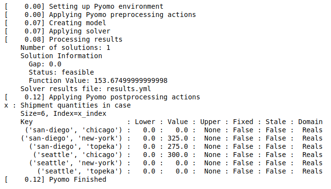
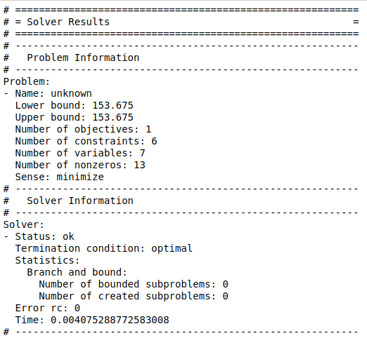
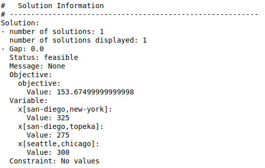
The numbers in square brackets indicate how much time was required for each step. Results are written to the file named results.yml, which as a special structure that makes it useful for post-processing.

This solution shows that the minimum transport costs is attained when 300 cases are sent from the Seattle plant to the Chicago market, 50 cases from Seattle to New-York and 275 cases each are sent from San-Diego plant to New-York and Topeka market.

The total transport costs will be $153.675

• Original problem formulation:
• Dantzig, G B, Chapter 3.3. In Linear Programming and Extensions. Princeton University Press, Princeton, New Jersey, 1963.
• GAMS implementation:
• Rosenthal, R E, Chapter 2: A GAMS Tutorial. In GAMS: A User's Guide. The Scientific Press, Redwood City, California, 1988.
• Pyomo translation: Antonello Lobianco