Description of the problem

Winton, a British investment management company, is looking to create novel statistical modelling and data mining techniques to predict stock returns.

Given historical stock performance and masked features, your task is to predict the end of day returns. The dataset contains 40000 random stock performance for a random 5-day period, days D-2, D-1, D, and D+1, which you can use to predict the returns in days D+2. The dataset also has 25 features, Feature_1 though Feature_25.

What you will build

• Linear regression
• Random forest regressor
• Gradient boosting regressor

What you will learn

• Perform exploratory data analysis (EDA) on data
• Clean large dataset for fitting the model
• Use models in sklearn to build, train data, tune hyperparameter and evaluate their performance

• pandas
• numpy
• matplotlib
• sklearn

First, use pandas pd.read_csv to read the csv file.

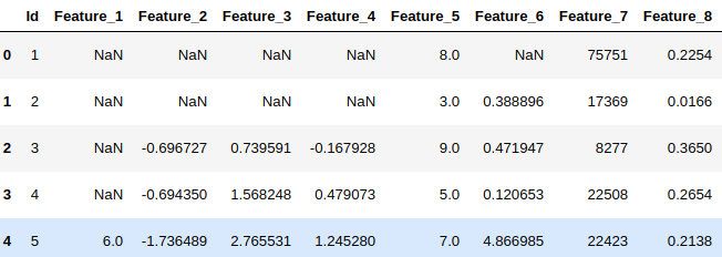
Let's look at the top 5 rows in the dataset (the columns are partly shown below):

Get the information of the dataset:

The dataset is 64.4MB with 40000 rows and 211 columns which are all numeric variables.

Exploratory Data Analysis (EDA) is an open-ended process where we calculate statistics and make figures to find trends, anomalies, patterns, or relationships within the data. EDA generally starts out with a high level overview, and then narrows into specific areas depending on your goals. It can help you with your modeling later on when you are deciding which features to use for your models.

In this dataset, there are two types of independent variables, one is the feature of stock, the other one is the returns of the stock. You can use different methods to plot those variables.

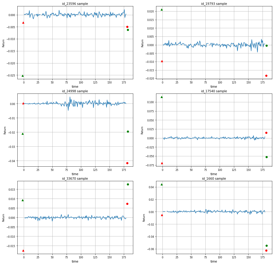
Below are randomly selected 6 stock samples by using line chart. Ret_2 to Ret_180 are returns over approximately one minute on day D. The red and green triangles indicate returns of D-1 (Ret_MinusOne) and D-2 (Ret_MinusTwo). Similarly, the red and green circles indicate D+1 (Ret_PlusOne) and D+2 (Ret_PlusTwo) respectively.

The green circle (Ret_PlusTwo: D+2) is the variable that you need to predict, but it seems that there is no significant relationship between D+2 and other return values.

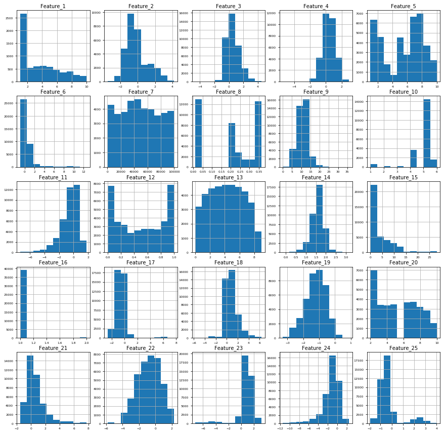
Now, plot the frequency distribution of each feature.

From these distribution plots, you can see that some features have normal distribution (e.g. Feature_2, Feature_3, Feature_4), while some features have outliers (e.g. Feature_6, Feature_16). By looking at all the histograms, you may have a better idea on how to fill in the missing values for the next step.

First, you may need to remove the columns with high percent (40%) of missing values ['Feature_1' 'Feature_10'].

For filling in missing values on numeric variables, you can apply the following methods by using Pandas' fillna() function.

• For Returns columns: Replace all the Nan values with mean value of the column
• For Feature columns: Replace all the Nan values with the most repeated value in that columns

Remove highly correlated predictors

Multicollinearity occurs when your model includes multiple factors that are correlated not just to your response variable, but also to each other. It may increase the standard errors of the coefficients which will make some variables statistically insignificant when they should be significant. In order to select actual significant features, you may need to remove highly correlated predictors from the model. Here, we can find the feature with correlation greater than 0.4.

Split the data into 70% train set and 30% test set, separate the dependent and independent variables. Since you will also use linear regression model to make predictions, it is a good idea to prepare a standardized data for it.

You can use the following metrics to evaluate different regression models:

• MAPE: Mean Absolute Percentage Error, also known as Mean Absolute Percentage Deviation (MAPD), is a measure of prediction accuracy of a forecasting method in statistics. It usually expresses accuracy as a percentage:
• 

where A represents the actual value and F is the forecast value

• MAE: Mean Absolute Error is a measure of difference between two continuous variables:
• 
• R^2 score: R^2 is a statistical measure of how close the data fits a regression line. It is also known as the coefficient of determination, or the coefficient of multiple determination for multiple regression.
• R^2 = Explained variation / Total variation. R^2 is always between 0 and 1.

From the evaluation of each basic model shown above, we can learn that GradientBoostingRegressor model has the best performance, where MAPE=1.36, R^2 score=0.05. However, this performance is not impressive, neither the R^2 score is. That's partly because it hasn't been tuned; selection of important features and hyperparameters is critical for machine learning modeling.

Select significant features

One method of feature engineering is to select the features with high importance.

In this dataset, most features have a low importance score. You can try to get rid of features with scores less than 0.001 first. Then, split the dataset, fit the model, get evaluation of the model again using those selected features.

All scores does not change too much. This means after removing those unimportant features, our model stay as good as before, and this is preferable. Given fewer number of features, this model would be more robust than the previous one. The result suggests that the model would potentially be fitting unseen data better.

Hyperparameter tuning

Hyperparameters is like the settings of an algorithm that can be adjusted to optimize performance. Sklearn implements a set of sensible default hyperparameters for all models, but these are not guaranteed to be optimal for a problem. The best hyperparameters are usually impossible to determine ahead of time, and tuning a model is where machine learning turns from a science into trial-and-error based engineering. Usually, the standard procedure for hyperparameter optimization accounts for overfitting through cross validation.

Result table

The best result is shown above, although MAPE and the average error, MAE slightly decrease, the increase in R^2 score is noticeable. This means hyperparameter tuning improves the performance of the model.

Kaggle.com The Winton Stock Market Challenge (2015) Retrieved from https://www.kaggle.com/c/the-winton-stock-market-challenge