Last Updated: 06/03/2020
What is a Variational Autoencoder (VAE)?
VAE is a generative model - it estimates the Probability Density Function (PDF) of the training data. If such a model is trained on, for example, time series data of Apple's stock price, it should assign a high probability value to any data point from Apple's stock price. A data point from some other time series, say Microsoft, on the other hand should be assigned a low probability value.
The VAE model can also sample examples from the learned PDF since it'll be able to generate new examples that look similar to the original dataset! This is what we are particularly interested in.
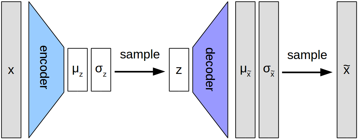
As seen from the figure, the input x is encoded into a smaller (technically, latent space) and then decoded back into original  . VAE learnt the distribution of the
  i.e.
i.e.  and
and  . For forecasting or generating synthetic data, we sample from this learnt distribution and decoders throws out the data.
Use Case
We use VAE for Univariate time series forecasting.
What will you build?
- A Variational Autoencoder for generating synthetic univariate time series data.
What will you learn?
- Preprocessing required for generation of synthetic time series
- How to make VAE model
- How to analyse various generated scenarios
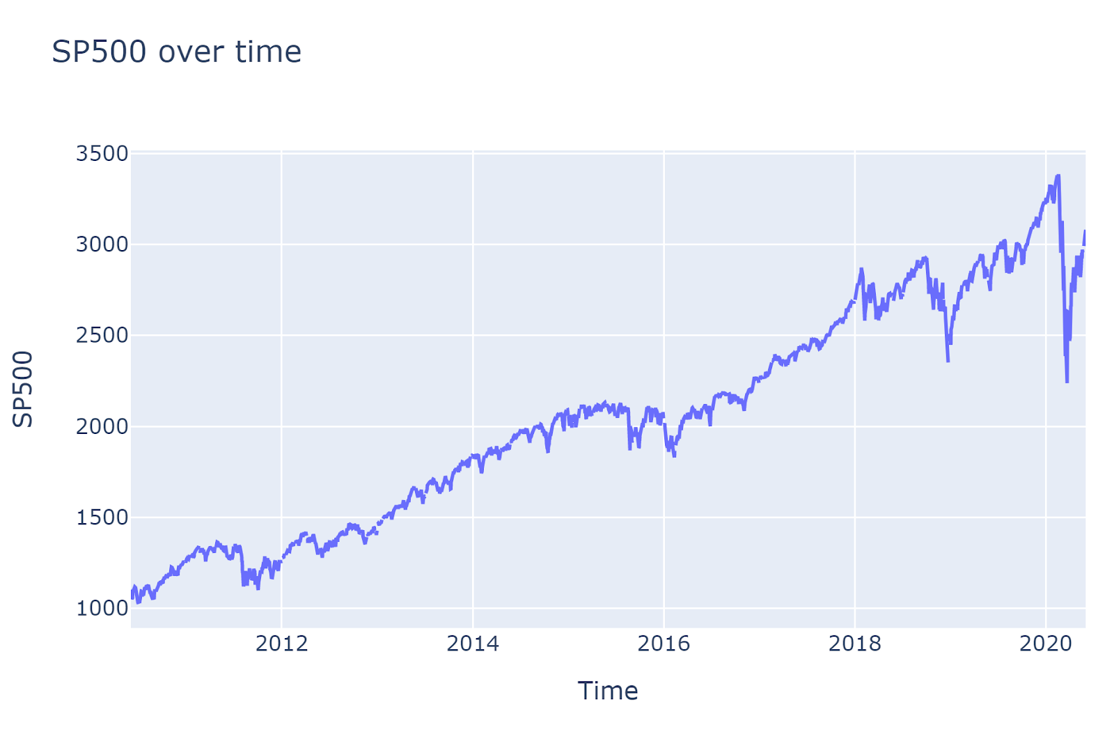
Getting Data
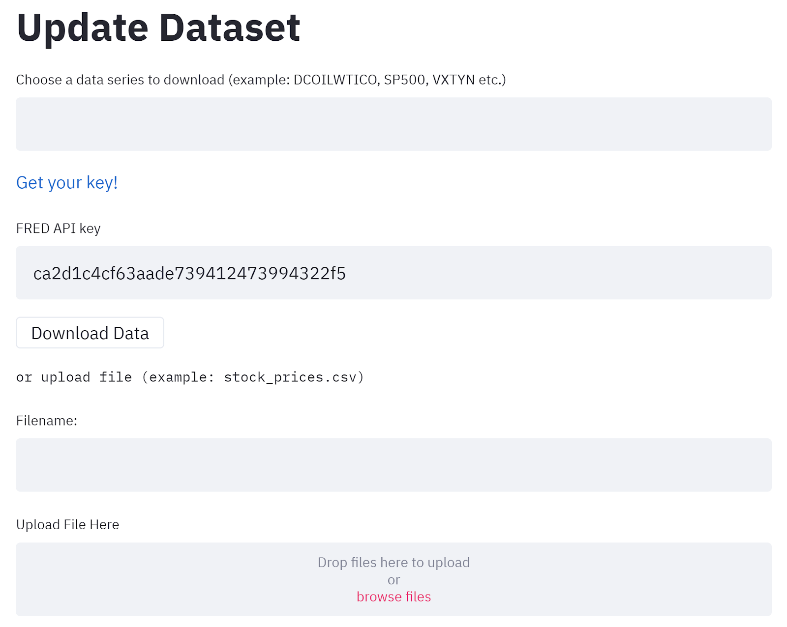
We can fetch the data in 2 possible ways:
- From FRED datasource (Learn more here)
- Uploading .csv file
The data has values (prices, indexes etc.) and corresponding timestamp.
Restructuring data for ingestion
Since we are dealing with time series data, data values might show some increasing/decreasing trends. In other words, they might not fall on the same scale. So, it is necessary to normalise the dataset.
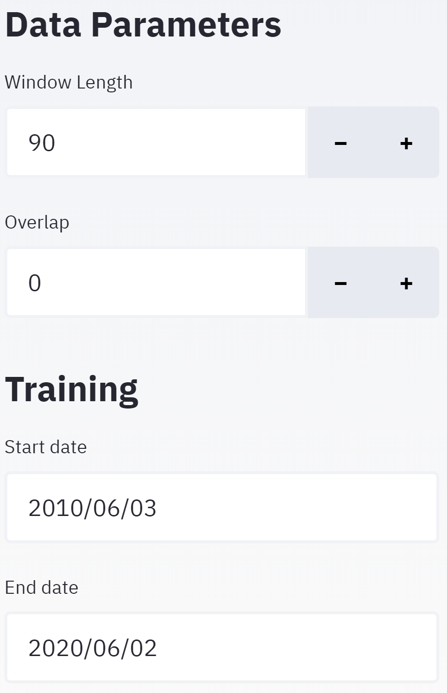
The preprocessing function normalises the value. Apart from this, it also provides functionality for clipping the data between start_date and end_date. You can also specify the window and overlap periods for restructure the data. In other words, you can restructure your 1-dimensional data into N sequences of window length with overlap days
| Window Length specifies how long the sequence should be i.e. how many days' of data should 1 sequence have. Whereas, overlap specifies how much each sequence should overlap For example, your data is A window length of, say 10, and overlap length of, say 0, would result in following restructured data: Sequence 1: Sequence 1: A window length of, say 10, and overlap length of, say 5, would result in following restructured data: Sequence 1: Sequence 1: Start and End date can be used to clip the dataset as per the usage. |
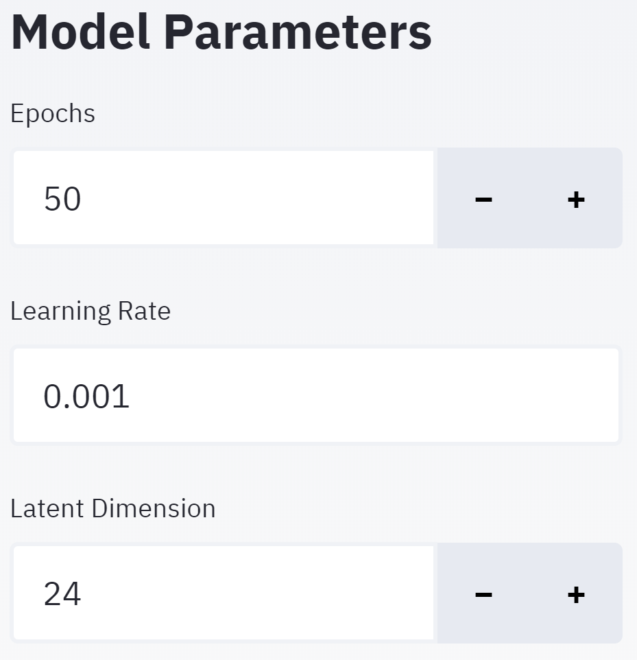
| Here you can define basic model parameters. Epochs specify how many passes should the model make over the dataset for learning. For faster training, the default value is set to 50. Learning rate is a tuning parameter in an optimization algorithm that determines the step size at each iteration Latent Dimension is specific to our VAE case. It specifies the latent or lower dimensional space. |
About model
The model comprises an encoder architecture and decoder architecture. As the name suggests, encoder encodes the data whereas the decoder decodes the data. Encoder reduces the data from original space to a much smaller sub-space. This results in a bottleneck structure. Later, the decoder decodes it back to the original space. The key point in VAE, which makes it different from vanilla autoencoders, is its latent subspace. While the encoder learns the  and
and  making up the subspace, the reparameterization step combines
  and
and  into a latent variable
  . This latent subspace, unlike vanilla autoencoders, is continuous. We can thus leverage this functionality and generate synthetic data.
Note: The encoder model is sometimes referred to as the recognition model whereas the decoder model is sometimes referred to as the generative model.
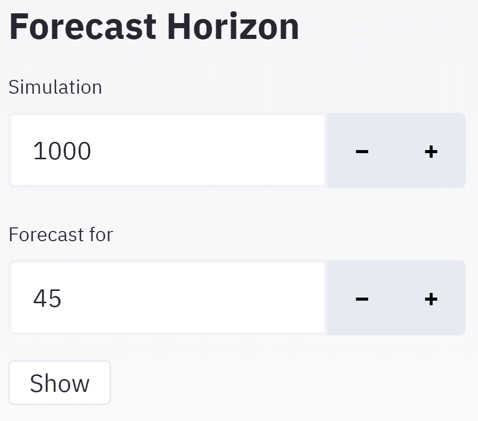
| Simulations specify the number of simulation you want to generate Forecast period specifies how much in future you want to forecast. (The maximum value can be the window length that you specified in the train module) |
This section includes analysis over simulation data, and divided into the following subsections:
- Simulation Samples
- Histogram/Distribution of observations at a single timestep, t (t=0 by default)
- Distributions of entire forecasting periods, represented by mean and standard deviation
- K-Means Clustering of Scenarios
- Hierarchical Clustering of scenarios
- Clustering Comparison
- Discriminative Score(coming soon)
- Predictive Score(coming soon)
- PCA(coming soon)
- tSNE(coming soon)
Let's look at some of the plots. The plots are generated using the S & P 500 index.
Note: The training date period is 2014.
Simulation Samples
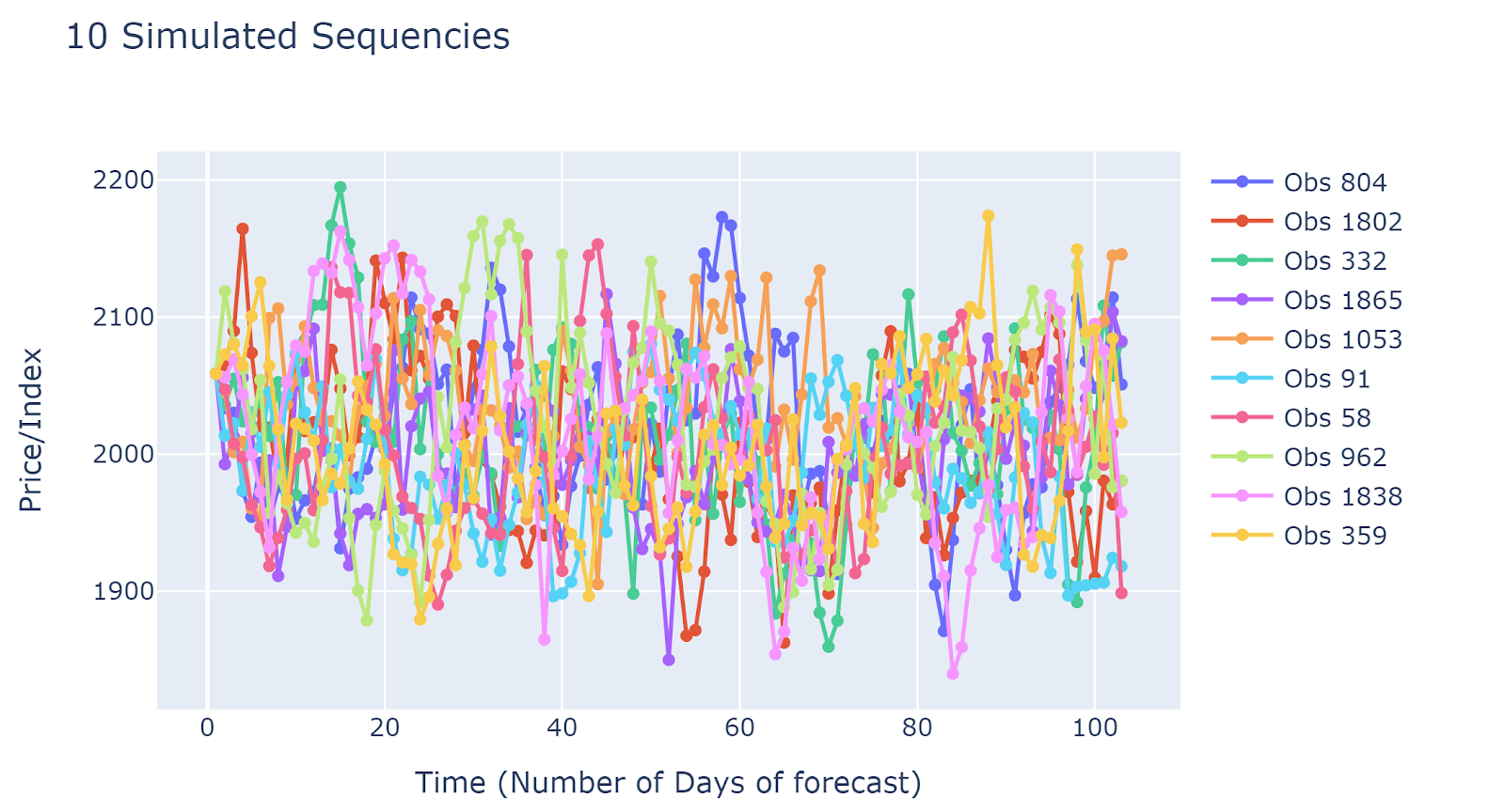
Simulated results are quite different from each other. This implied that the simulation results may capture many different scenarios. The disadvantage would be due to the large number of simulated sequences, it is hard to have generalized insights.
Histogram/Distribution of observations at a single timestep
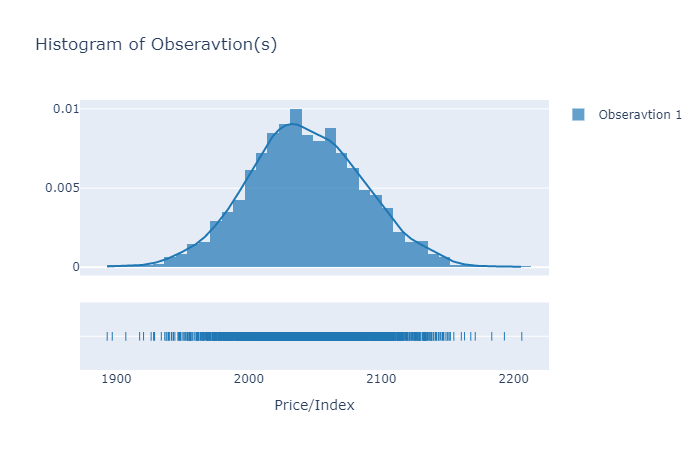
It is recommended to plot the histogram of the first time point. If it is distributed around the latest realized value (prices/index), then at least we can say that simulated data is not unrealistic.
K-Means Clustering of Scenarios
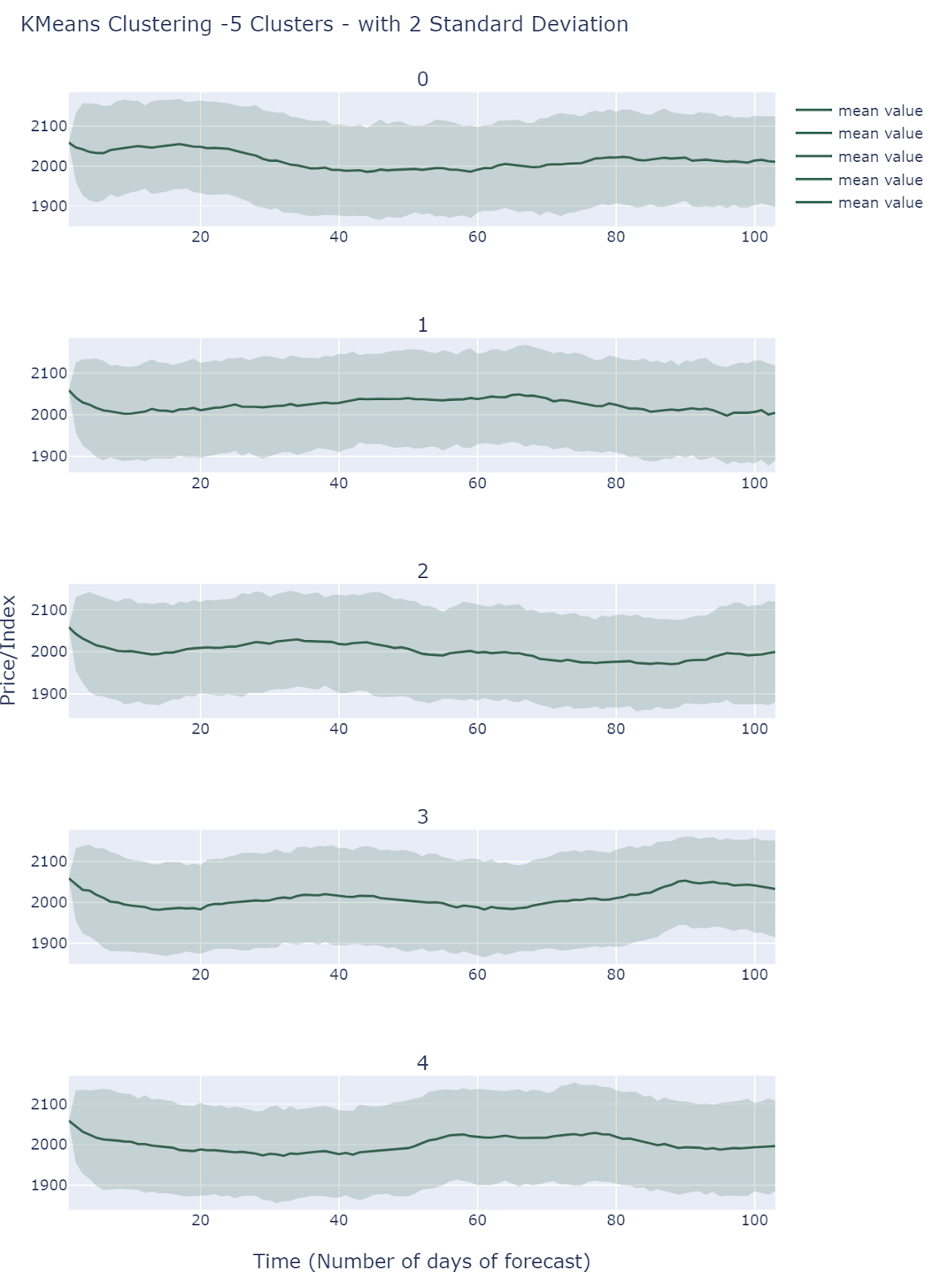
By default , we choose 5 clusters using L2-K-Means clustering to extract different scenarios.
All Clusters behave differently and they all fall into comparable ranges. Simulations does show different scenarios but it is still unclear how to interpret these results.
Hierarchical Clustering of scenarios
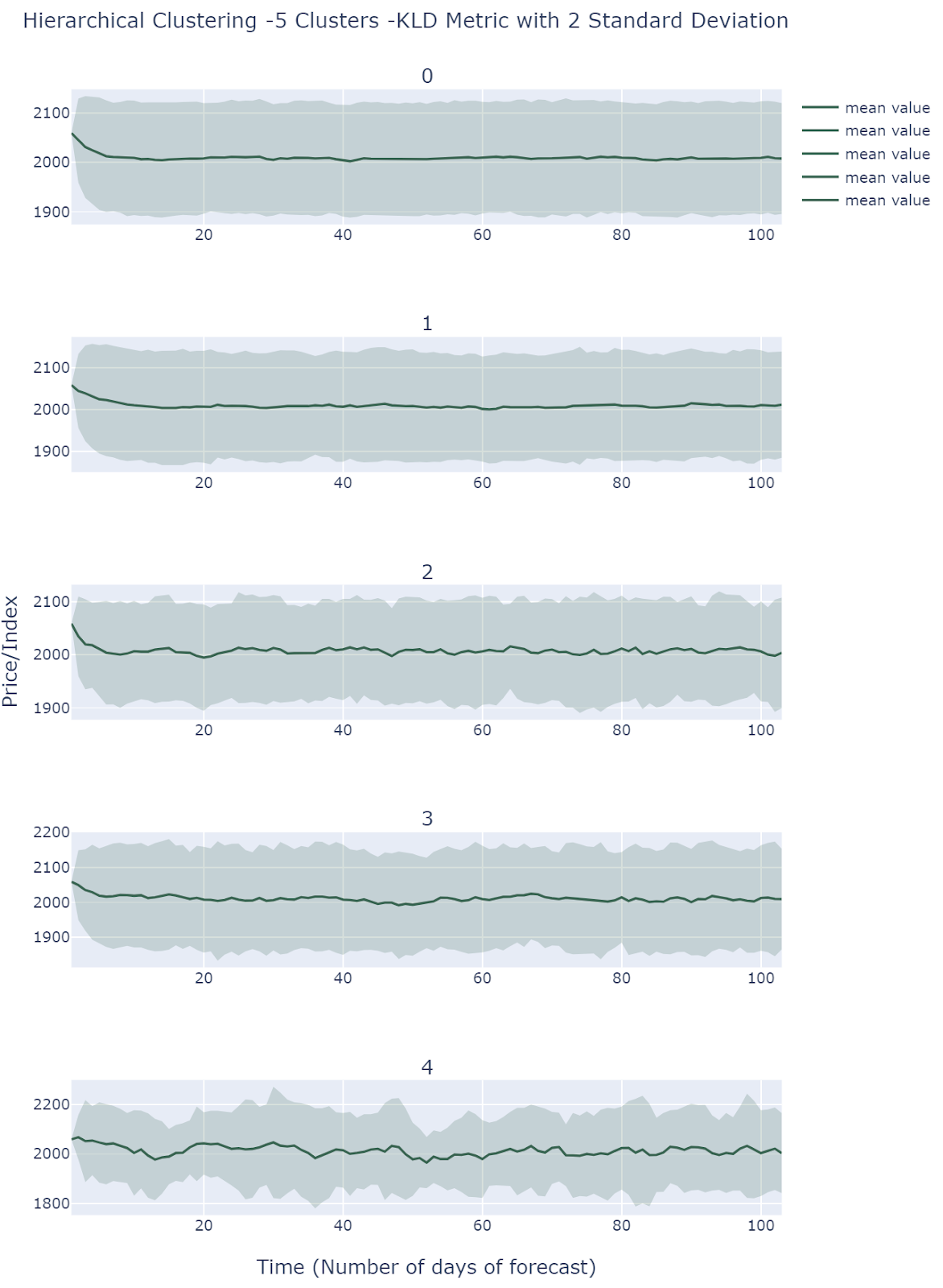
By default , we choose 5 clusters using Hierarchical Clustering(KL Divergence Affinity) to extract different scenarios. Cluster 0 and 1 presents relatively low volatilities, and cluster 2 and 3 shows medium volatilities. Cluster 4 is the most volatile one among all clusters. Therefore, Hierarchical Clustering method groups observations based on volatility.
 .
.
Clustering Comparison
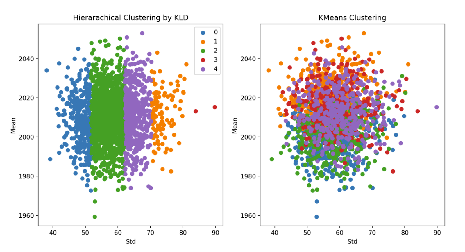
It is impossible and meaningless to analyze each sequence of simulated Price. Instead, we should focus on some 'major' pattern reflected by the simulated data. In order to capture the 'major' pattern from simulation results, KMeans(L2 distance) and Hierarchical Clustering(KL Divergence Affinity) are applied, and Line Area charts would be implemented for each cluster.
Each cluster could be regarded as a potential scenario for Price. If viewed this way, further scenario analysis could be done for different clusters, which may lead to robust decision making.


 and so on.
 and so on.